三周看了两篇 Biometrika,此前还没见过 spectral clustering,写总结发现很多地方完全理解错误,真是令人感叹(
下次还是一边看一边写吧,感觉可以少花点时间,但好像又不保证能发现一开始理解错的地方((
Background
General Basic Settings
In Network-Adjusted Covariates for Community Detection and Local Linear Graphon Estimation Using Covariates we consider unweighted, undirected network data with node-wise covariates.
Basic settings are represented as follows.
A network data is often represented as a graph \(\mathcal A = (\mathcal V, \mathcal E)\), where \(\mathcal V\) denotes the set of \(n\) nodes, and \(\mathcal E\) denotes the set of edges between nodes. The adjacency matrix \(A \in \{0,1\} ^{n \times n}\) shows the structure of the graph, where \(A_{ij} = A_{ji} =1\) if \((i,j) \in \mathcal E\) and \(A_{ij} = A_{ji} =0\) otherwise. Note that self-loop is not allowed, then \(A_{ii} = 0\) holds for any node \(i \in [n]\) (here \([n] = \{1,2, \cdots, n\}\) for simplexity). Let \(d_j = \sum_{j=1}^n A_{ij}\) denote the degree of node \(i\) and \(\bar d = \sum_{i=1}^n d_i/n\) be the average degree of the graph.
For a statistical network with node-wise covariates, denote the covariate vector of node \(i \in [n]\) as \(x_i \in \mathbb R^p\). Then the covariate matrix \(X \in \mathbb R^{n \times p}\) is constructed with the \(i\)-th row in \(X\) as \(x_i\).
Community Classifying
In a community classifying process, let \(K\) be the number of communities. Define a \(n\)-vector as the community label vector \(l \in [K]^n\) by denoting \(l(i) = k\), if the node \(i\) is in the \(k\)-th community. This can also be represented in the matrix form \(\Pi \in \{0,1\}^{n \times K}\) (which will be used to construct the Laplacian matrix), where \(\Pi_{ij} =1\) if \(l(i) = j\), i.e. node \(i\) is a member of community \(j\). We aim to recover \(\Pi\) in the classification problem.
Spectral Clustering Method & K-mean Clustering Method
I hadn't learned these two methods before, so I took some notes.
Compactness and Connectivity
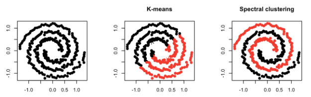
Firstly, we need to distinguish between two concepts - compactness and connectivity.
Compactness --- Points that lie close to each other fall in the same cluster and are compact around the cluster center. The closeness can be measured by the distance between the observations. E.g.: K-Means Clustering
Connectivity --- Points that are connected or immediately next to each other are put in the same cluster. Even if the distance between 2 points is less, if they are not connected, they are not clustered together. Spectral Clustering is a technique that follows this approach.
Principle of K-means Clustering
K-means stores \(k\) centroids that it uses to define clusters. A point is considered to be in a particular cluster if it is closer to that cluster's centroid than any other centroid. K-Means finds the best centroids by alternating between (1) assigning data points to clusters based on the current centroids and (2) choosing centroids (points which are the center of a cluster) based on the current assignment of data points to clusters.
The algorithm is shown below.
Algorithm 1 Repeat until convergence:{
For every \(i \in [n]\), set \(c^{(i)} = \arg \min _j \| x^{(i)} - \mu_j\|^2\);
For each \(j \in [k]\), set \(\mu_j = \frac{\sum_{i=1}^n \mathbf{1}_{c^{(i)} = j}x^{(i)}}{\sum_{i=1}^n \mathbf{1}_{c^{(i)} = j}}\). }
Principle of Spectral Clustering
Denote \(D = \text{diag} \{d_1,d_2,\cdots, d_n\}\) as the degree matrix, \(A\) as the adjacency matrix. Then the Laplacian of the graph is denoted as \(L = D-A\).
Note that for any \(f \in \mathbb R^n\), we have
\[\begin{aligned} \frac{1}{2} \sum_{i=1}^n \sum_{j=1}^n A_{ij} (f_i - f_j)^2 & =\frac{1}{2}( \sum_{i=1}^ n (\sum_{j=1}^n A_{ij})f_i ^2 + \sum_{j=1}^ n (\sum_{i=1}^n A_{ij})f_j ^2 - 2\sum_{i=1} \sum _{j=1} A_{ij} f_i f_j ) \\ &= \sum_{i=1} d_i f_i^2 - \sum_{i=1}^n \sum_{j=1}^n f_i f_j A_{ij} = f^T Df - f^T Af = f^T L f. \end{aligned}\]
Consider minimizing \(\frac{1}{2} \sum_{i=1}^n \sum_{j=1}^n A_{ij} (f_i - f_j)^2 = f^T L f\) under the embedding \(f^TDf =1\). (From the perspective of solving the min-cut problem, it's equivalent to minimizing \(\frac{f^T L f}{f^TDf}\).)
The Lagrangian is \(L(\lambda ; f) = f^TLf - \lambda f^T Df = f^T(L-\lambda D)f\). By differentiating w.r.t. \(f\), it is equivalent to solve \((L-\lambda D)f =0\), i.e. to solve the eigenvalues and eigenvectors of \(L^\prime = D^{-1}L = I - D^{-1} A\).
The algorithm of spectral clustering is listed below.
Algorithm 2 1. Compute \(D = \text{diag}\{d_1, \cdots, d_n\}, L^\prime = I - D^{-1} A\).
Compute the first \(K\) eigenvectors \(v_1,v_2, \cdots , v_K\) of the matrix \(L^\prime\).
Build the matrix \(V \in \mathbb R^{n \times K}\) with the \(K\) eigenvectors as columns.
Interpret the rows of \(V\) as new data points \(Z_i \in \mathbb R^K\).
Clustering the points \(Z_i\) with \(K\)-means clustering in \(\mathbb R^K\).
Graphon Function
In classical graphon theory, a graphon is a bivariate and symmetric \([0,1]\)-valued function \(f(u,v): [0,1] ^2 \to [0,1]\) defined on a probability space. In particular, the graphon model can be formulated as a data-generating process through the following two successive steps.
First, we draw the node-specific latent quantities \(\xi_1, \xi_2, \cdots , \xi_n\) i.i.d. \(\sim\) Uniform \([0,1]\).
Secondly, condition on the realizations of the latent quantities, i.e. given \(\xi_1, \xi_2, \cdots, \xi_n\), the adjacent matrix items follow certain conditional distribution as
\[A_{ij} | \xi_i , \xi_j \sim \text{Bernoulli} (f(\xi_1, \xi_j)),\]
where the graphon \(f\) satisfies \(f(u,v) = f(v,u)\) for any \((u,v) \in [0,1]^2\).
The Local Linear Graphon Estimation Using Covariates introduces some adjustments to the graphon function, to make emphasis the effect of \(n\) and node heterogeneity.
Stochastic Block Model
The stochastic block model is actually a construction of the graphon estimation, i.e., the graphon \(f\) is formulated as a piecewise constant step function with a rectangular pattern, i.e.
\[f(u,v) = \sum_{i=1}^K \sum_{j=1}^K \mathbf{1}_{\{\zeta_{i-1} \leq u < \zeta_i\}} \mathbf{1}_{\{\zeta_{j-1} \leq v < \zeta_j\}} P(i,j).\]
Specifically, for node pair \((i,j)\) from community \((l(i),l(j))\), the distribution of \(A_{ij}\) is
\[A_{ij} | l(i), l(j) \sim \text{Bernoulli}( P(l(i),l(j))).\]
In Network-Adjusted Covariates for Community Detection, we utilize the degree-corrected stochastic model concerning the popularity of each node. The degree-corrected graphon is represented as:
\[f(u, \cdot) = a_k(u) w(\zeta_{k-1}, \cdot) \; \text{for all }u \in (\zeta_{k-1}, \zeta_k),\]
where \(a_k : [0,1] \to \mathbb R_+\) is a continuous non-decreasing function with \(a_k(\zeta_{k-1}) =1\). This setting entails that two nodes from the same group will reveal the same basic connectivity behavior (stochastically) but differ in the expected degree by introducing \(a_k\) for each community \(k \in [K]\).
Specifically, for node pair \((i,j)\) from community \((l(i),l(j))\), the distribution of \(A_{ij}\) is
\[A_{ij} | l(i), l(j) \sim \text{Bernoulli}( \theta _i \theta _j P(l(i),l(j))),\]
where the coefficient \(\theta_i\) represents the popularity of node \(i\) itself.
Denote \(\Theta = \text{diag} \{\theta_1, \cdots, \theta_n\} \in \mathbb R^{n \times n}\), \(P = \{ P(i,j)\}_{n \times n} \in \mathbb R^{n \times n}\), and the adjacency matrix \(A\) can be identified by
\[E(A |\Pi) = \Omega_A - \text{diag} (\Omega _A), \; \Omega_A = \Omega \Pi P \Pi^T \Theta.\]
Here the subtraction of \(\text{diag}(\Omega_A)\) is to eliminate self-loops in the network.
Covariates Modelling
To highlight the integrity of the network model, we always start from a simple situation: the total model scale is large, and the mean degree is dominated by dense communities. In the subsequent analysis, we have drawn two intuitive conclusions from this.
The adjusted covariates of nodes in different communities are affected by \(\sum_{j: A_{ij}=1} x_j\) and \(\alpha_i x_i\), respectively. Furthermore, when \(x_i \sim ^{\text{approx}} F_D, x_j \sim ^{\text{approx}} F_S, i \in D, j \in S\) is true, the results obtained using spectral clustering exhibit similar central distributions.
Thus, we keep this setting and adjust it similarly to a community-wise identity distribution setting, i.e. the covariates \(x_i\) are generated by a standard clustering model, and they are independently distributed as
\[x_i | \Pi \sim F_k, \; l(i) = k \in [K].\]
Moreover, we assume that given the label vector \(l\), \(X\) is independent of \(A\).
Block Assignment According to Bandwidth
Given a suitable bandwidth \(1 < h \leq n\), denote \(n = kh + r\) where \(r \equiv n \pmod h\). Then we assign \(n\) nodes into \(k\) blocks, with the first \(k-1\) blocks having \(h\) nodes each, and the last block has \(h+r\).
To represent this assignment, let \(\mathcal Z_{n,h} \subseteq [k]^n \subset \mathcal R^n\) contain all block assignment vectors \(z = (z_1, \cdots, z_n)^T\), where \(z_i = j\) implies that node \(i\) is in the \(j\)-th block, \(1 \leq i \leq n, 1 \leq j \leq k\).
Actually, in Local Linear Graphon Estimation Using Covariates we assign oracle into \(k\) blocks with order statistics.
Network-Adjusted Covariates for Community Detection
This work introduces a network-adjusted covariate (based on the community density) and applies the spectral clustering method to the adjusted covariate matrix in two ways according to the different inputs. Through orthogonal matrix transformation, the error between the two outputs can be controlled. This indicates that this method has good consistency.
Network-Adjusted Covariates
This work introduces a network-adjusted covariate \(\{y_i\}\) based on the effect of community density and the node-wise covariates \(\{x_i\}\):
\[y_i = \alpha_i x_i + \sum_{j : A_{ij} =1} x_j, \; \forall x \in [n],\]
and the weight
\[\alpha _i =\frac{\bar d /2}{d_i / \log n +1}\] is
chosen to balance the effect of neighbors (i.e., \(\sum_{j \neq i} x_j\).
This seems reasonable because neighbors are the most likely potential members of the community that \(i\) is in), and the effect of the node itself (i.e. \(x_i\)) according to the density of community it is in.
To see how \(\alpha_i\) balance two parts, we need to define the sparsity and density of a certain community.
Definition 2.1 (Sparse/Dense Community). Consider a network \(\mathcal A = (\mathcal V, \mathcal E)\) and constants \(c_d > c_s >0\). Consider community \(k\), we call it a
(Relatively) dense community, if \(E(d_i) \geq c_d \log n\) for any node \(i\) s.t. \(l(i) = k\) (i.e. node \(i\) is a member of the community \(k\)).
(Extremely) sparse community, if \(E(d_i) \leq c_s \log n\) for any node \(i\) s.t. \(l(i) = k\) (i.e. node \(i\) is a member of the community \(k\)).
This definition will be slightly adjusted later according to the stochastic block model.
Question: Why we can assume that the \(K\) communities are either sparse or dense ones (according to the setting in the paper)?
I think this assumption can be satisfied through proper selection of \(c_D, c_S\) (in extreme cases they are almost the same), but this will somehow weaken the definition. Or this is just an assumption on the network structure itself. (unimportant)
Intuitively, we consider the case where the community sizes are comparable, then the average degree \(\bar d\) is dominated by dense communities. Then for node \(i\) in dense communities we have \(\alpha _i \approx \log n /2 < n\), then the focus of weighting was on \(\sum_{j : A_{ij}=1} x_j\), i.e. the potential community members of node \(i\). Similarly, for node \(i\) in sparse communities, we have \(\alpha _i \geq \frac{\bar d /2}{c_S +1} \approx \frac{c_D}{2(c_S+1)} \log n\), which will let \(\alpha _i x\) be considerably large with respect to \(\sum_{j : A_{ij}=1} x_j\).
Therefore, for nodes in dense communities, the adjusted covariates focus on connections with potential community members to imply density. And for sparse community members, the emphasis should be put on the node itself because the network may not give much meaningful information.
Let \(Y = (y_1 ,\cdots , y_n)^T\) be the network-adjusted covariate matrix, then \[Y = AX + D_\alpha X = (A+D_\alpha)X,\] where \(A\) is the adjacency matrix, \(X\) is the covariate matrix, and \(D_\alpha = \text{diag} \{\alpha_1, \cdots, \alpha_n\}\) as the matrix of weights.
Direct Spectral Clustering
Here the graph \(\mathcal A = (\mathcal V, \mathcal E)\), the adjacent matrix \(A\) and the covariates \(X\) are known. We operate the spectral clustering method on the network-adjusted covariates \(Y\) (also the generalized form) to give an estimated community assignment \(\hat l(i)\), \(i \in [n]\).
Spectral Clustering on Network-Adjusted Covariates
We can apply the spectral clustering method to the network-adjusted covariate matrix \(Y\) directly when \((A,X)\) are both known. The algorithm is shown below.
Algorithm 3 1. Compute \(Y = AX + D_\alpha X\).
Compute the first \(K\) normalized left singular vectors \(\hat \xi_1,\hat \xi_2, \cdots , \hat \xi_K\) of the matrix \(Y\).
Build the matrix \(\hat \Xi \in \mathbb R^{n \times K}\) with the \(K\) eigenvectors as columns.
Interpret the rows of \(\hat \Xi\) as new data points \(\hat Z_i \in \mathbb R^K\).
Clustering the points \(\hat Z_i\) with \(K\)-means clustering in \(\mathbb R^K\), and get the community label vector \(\hat l\) according to the result.
Note that the network-adjusted covariates are dominated by \(\sum_{j: A_{ij}=1} x_j\) for node \(i\) in dense communities, and by \(\alpha_i x_i\) for \(i\) in sparse communities. Then for the large-scale community condition, we considered in the previous section, for node \(i\) in dense communities, \(y_i \approx \sum_{j :A_{ij}=1} x_i \approx d_i F_D\) if \(\{x_i\}_{i \in D}\) follows similar distribution. Similarly, for node \(i\) in sparse communities, \(y_i \approx \alpha_i x_i \approx \frac{c_D}{2(c_S+1)} \log n F_S\) if \(\{x_i\}_{i \in S}\) follows similar distribution.
Hence, the central distribution of adjusted covariates is approximately the same up to degree heterogeneity factor \(d_i\) in dense communities and constant factor in sparse communities. This consistency will be inherited by the left singular matrix \(\hat \Xi\), and so are the rows of \(\hat \Xi\), which is used as data in k-mean clustering.
Spectral Clustering on Generalized Adjusted Covariates
In the case the covariate matrix \(X\) is uninformative, it should not be included in the spectral clustering matrix \(Y = (A+D_\alpha )X\). Then we leverage \(YY^T\) with the adjacency matrix \(AA^T\), by denoting the "Laplacian matrix" as \(L = YY^T + \beta n AA^T\) and performing the spectral clustering algorithm as follows.
Algorithm 4 1. Compute \(Y = AX + D_\alpha X\), \(L= YY^T + \beta n AA^T\).
Compute the first \(K\) normalized left singular vectors \(\hat \xi_1,\hat \xi_2, \cdots , \hat \xi_K\) of the matrix \(L\).
Build the matrix \(\hat \Xi \in \mathbb R^{n \times K}\) with the \(K\) eigenvectors as columns.
Interpret the rows of \(\hat \Xi\) as new data points \(\hat Z_i \in \mathbb R^K\).
Clustering the points \(\hat Z_i\) with \(K\)-means clustering in \(\mathbb R^K\), and get the community label vector \(\hat l\) according to the result.
\(\beta\) is selected as \(\| \hat x\|^2\). Actually larger \(\beta\) is often preferred.
Degree-Corrected Stochastic Blockmodel
According to the basic settings in the Background section, we apply the degree-corrected stochastic block model with known parameters \((\Theta, K, P, \Pi, F_{[K]})\) here as follows. Note that \((A,X)\) are unknown and will be estimated by their mean. Also, \(\mathcal D, \mathcal S\) are both unknown as a basic setting.
Basic Ideas: This is another way to perform the clustering, but the adjacent matrix \(A\) and the covariate matrix \(X\) are both unknown. However, \((\Theta, K, P, \Pi, F_{[K]})\) are known parameters. We replace both of them with their expectation to get the estimated network-adjusted covariate matrix \(\hat Y\) used for spectral clustering, which can be calculated under the setting of a degree-corrected stochastic block model.
Then we're going to compare the output with \(\hat l\) estimated by \((A,X)\) previously, and show that there exists consistency even though the inputs are totally different (one with \((\mathcal A,X, A)\) and another with \((\Theta, K, P, \Pi, F_{[K]})\)). This implies that the spectral clustering on network-adjusted covariates is powerful.
Moreover, there may be mis-specified nodes in the given community membership matrix \(\Pi\). We'll show that the spectral clustering method on network-adjusted covariates will correct some of them.
The process is shown as follows.
Model Establishment and Spectral Clustering
For node pair \((i,j)\) from community \((l(i),l(j))\), the distribution of \(A_{ij}\) is
\[A_{ij} | l(i), l(j) \sim \text{Bernoulli}( \theta _i \theta _j P(l(i),l(j))),\]
where the coefficient \(\theta_i\) represents the popularity of node \(i\) itself.
Denote \(\Theta = \text{diag} \{\theta_1, \cdots, \theta_n\} \in \mathbb R^{n \times n}\), \(P = \{ P(i,j)\}_{n \times n} \in \mathbb R^{n \times n}\), and the adjacency matrix \(A\) can be identified by
\[E(A |\Pi) = \Omega_A - \text{diag} (\Omega _A), \; \Omega_A = \Omega \Pi P \Pi^T \Theta.\]
Moreover, we suppose that \(X\) is independent of \(A\) given the label vector \(l\) as a covariate modeling assumption, i.e. they are independently distributed as
\[x_i | \Pi \sim F_k, \; l(i) = k \in [K].\]
A standard stochastic block model generates the covariates \(x_i\) according to the \(F_{[K]}\), and the estimation of \(X\) we use later is
\[E(X) = [E(x_{i})]_{i \in [n]} = [E(F_{l(i)})]_{i \in [n]}.\]
Under the above settings, note that
\[E(d_i) = E(\sum_{j=1}^n A_{ij}) = \theta _i \sum_{j \neq i} \theta_j P(i,j) \leq n \theta_i \max_{i \in [n]}\{\theta_i\},\]
we refine the definition of dense and sparse communities by approximating the degree with the upper bound \(n \theta_i \theta_{\text{max}}\) as follows.
Definition 2.2 (Sparse/Dense Community Adjusted for Stochastic Blockmodel). Consider a network \(\mathcal A = (\mathcal V, \mathcal E)\) that follows the degree-corrected stochastic blockmodel with parameters \((\Theta, K,P, \Pi, \theta)\) and \(\theta_{\text{max}} = \|\theta \|_{\infty}\). Consider community \(k\), we call it a
(Relatively) dense community, if there exist constants \(c,c_d\) s.t. \(\theta _i \geq c \theta_{\text{max}}\), and \(n \theta _i \theta_{\text{max}} \geq c_d \log n\) for any node \(i\) s.t. \(l(i) = k\) (i.e. node \(i\) is a member of the community \(k\)).
(Extremely) sparse community, if there exist constants \(0<c_s < c_d\) \(n \theta_i \theta_{\text{max}} \leq c_s \log n\) for any node \(i\) s.t. \(l(i) = k\) (i.e. node \(i\) is a member of the community \(k\)).
Question: Here \(E(d_i) = \theta _i \sum_{j \neq i} \theta_j P(i,j)\) is dominated by \(n \theta_i \| \theta \|_{\infty}\), however this is a bit rough. We can replace this upper bound by \(\theta_i \sum_{i=1} ^n = \theta _i \| \theta \|_1\). Will this make much difference? (I think not.)
To set up an oracle matrix for the network-adjusted covariate matrix, we consider the dominated terms only. If \(i \in \mathcal D\), the dominated term of \(y_i\) is \(\sum_{j : A_{ij} =1} x_j\), which can be estimated by the i-th row of \(E(A) E(X)\). If \(i \in \mathcal S\), the dominated term of \(y_i\) is \(\alpha_i x_i\), which can be estimated by the i-th row of \(\hat \alpha_i E(X)\). Here the estimated weight is
\[\hat \alpha_i = \frac{E(\bar d) \log n}{2(E(d_i) + \log n)}.\]
Denote \(I_{\mathcal D}\) as the identity matrix where only diagonals on \(\mathcal D\) are preserved and others are set as 0. This definition can be extended to other matrices. Hence
\[\Omega = \hat Y = (I_{\mathcal D} E(A) I_{\mathcal D})E(X) + I_{\mathcal S} \hat D_\alpha E(X) = (I_{\mathcal D} E(A) T_{\mathcal D} + I_{\mathcal S} \hat D_\alpha) E(X)\]
is the "network-adjusted covariate matrix" under population settings, where \(\hat D_\alpha = \text{diag} \{\hat \alpha _1, \cdots, \hat \alpha_n\}\).
Mis-specifying of Nodes and Recovery Methods
Under the setting of the degree-corrected stochastic block model, we define mis-specifying by the distribution of \(x_i\). Note that the conditional distribution of \(x_i | \Pi\) is denoted as \(F_k\) for \(l(i) = k\). However, the membership in \(\Pi\) may be wrong, which causes mis-specifying and will result in:
\[x_i | \Pi \sim F_k, \; \; \text{but } x_i \sim G_i \neq F_k.\]
Such nodes \(x_i\) are called mis-specified nodes, and the corresponding row in \(E(X)\) will be affected by such error. The set of mis-specified nodes is denoted as \(\mathcal M\).
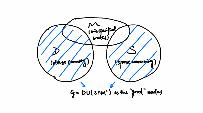
Though the set \(\mathcal D, \mathcal S\) are unknown, we can classify the nodes into the three sets above. Denote \(\mathcal G = D \cup (S \cap M^c)\) as the "good" nodes that can be recovered (this is guaranteed by Theorem 2.2).
Similar to the process of directly applying spectral clustering to \(Y\), we consider the adjusted covariates and the generalized adjusted covariates as follows.
Oracle Based Network-Adjusted Covariate Clustering
Consider the spectral clustering on the oracle matrix \(\Omega _{\mathcal G} = I_{\mathcal G} \Omega\), we have the following lemma.
Lemma 1 (Spectral Analysis on Oracle Matrix). Consider \(\Omega_{\mathcal G} = I_{\mathcal G} \Omega\) as the oracle matrix with rows restricted on \(\mathcal G\). Denote the singular value decomposition of \(\Omega _{\mathcal G}\) as \(\Omega_{\mathcal G} = \Xi \Lambda U^T\), where \(\Xi \in \mathbb R^{n \times K}, U \in \mathbb R^{p \times K}\), and \(\Lambda \in \mathbb R^{K \times K}\). Then there is
\[\Xi_ i = \begin{cases} \theta _i v_{l(i)}, \; & i \in \mathcal D \\ \hat \alpha_i u_{l(i)}, \; & i \in \mathcal S \cap \mathcal M^c \\ 0 , \; & i \in S \cap M = \mathcal G^c, \end{cases}\]
where \(\{v_k\}\)'s and \(\{u_k\}\)'s are \(K\)-dimensional vectors.
Question: This is just an oracle analysis even based on known \(\mathcal M\), how can we reach the conclusion that "the label of nodes in \(\mathcal G\) can be exactly recovered"?
I think by "recovery" the author means that, under the setting of the stochastic block model, even if there are some mis-specified nodes in \(\Pi\) (i.e. the distribution of covariates \(x_i\) is wrongly assigned as \(F_{l(i)}\)), \(\hat l(i)\) and \(\Pi_{i,j}\) can correspond to each other for nodes in \(\mathcal G\).
The lemma implies that by separating the centers (i.e. \(u_k\) 's and \(v_k\) 's), the label of nodes in \(\mathcal G\) can be exactly recovered. Actually, the central distribution can be identified through the orthogonal transformation between \(\hat \Xi\) and \(\Xi\) with high probability and slight error. This can be guaranteed by the following theorem.
Theorem 2.1 (Row-wise empirical and oracle singular matrix distance). Consider the degree-corrected stochastic block model with covariates with parameters \((\Omega, K, P, \Pi , F_{[K]}, \mathcal M)\), where \(p>0\) is constant, \(\mathcal G\) is the set of good nodes and \(\varepsilon = |\mathcal G^c| /n\). Let \(\Omega\) be the oracle matrix, \(\Xi\) is the left singular matrix of \(\Omega_{\mathcal G} = I_{\mathcal G} \Omega\), and \(\hat \Xi\) consists of the top \(K\) left singular vectors of \(Y\).
Let \(c,C>0\) be constants that vary case by case. We assume:
the sub-matrix of \(P\) that restricted to dense communities \(P_{\mathcal D} = I_{\mathcal D} P\) is full-rank;
\(\| x _i \| \leq R\) almost surely, and for \(i \in \mathcal S \cap \mathcal G\), with high probability \(\| x_i \ E(x_i)\| \leq \delta_X R\);
\(\lambda _K E(X) \geq c \sqrt n R\);
the number of nodes in any community \(n_k / n \geq c >0\).
Then there are threshold constants \(C_\theta, \varepsilon _0, n_0\), and \(\delta_0\), s.t. if \(\delta_X \leq \delta _0\), \(\varepsilon \leq \varepsilon_0\), \(n \geq n_0\), \(n \theta_{\text{max}}^2 \geq C_\theta \log n\), there exists an orthogonal matrix \(O\) and a constant \(C>0\) with probability \(1 - O(1/n)\) s.t.
\[\max _{i \in \mathcal G} \|\hat \Xi_i - O \xi_i\| \leq C(\delta_X + \sqrt \varepsilon + 1/ \sqrt{C_\theta}) / \sqrt{n},\]
where \(\hat \Xi_i\) and \(\Xi_i\) are vectors formed by i-th row of \(\hat \Xi\) and \(\Xi\).
Hence, the algorithm of spectral clustering based on network-adjusted covariates shows strong consistency. \(\hat l(i)\) and \(\Pi_{i,j}\) can correspond to each other for each node in the good set \(\mathcal G\). Note that the bound is row-wise instead of the Frobenius norm bound using the Davis-Kahan approach (haven't read yet).
Theorem 2.2 (Strong Consistency). Suppose the conditions 1 \(\sim\) 4 in Theorem 2.1 hold. Let \(\hat l\) be the estimated labels by the spectral clustering method in \(Y\). Then there is a constant \(C_\theta\) independent of \(n\), so that if \(n \theta_{\max} \geq C_\theta \log n\), there exists a permutation \(\pi\) s.t. with probability \(1- O(1/n)\),
\[\pi(\hat l(i)) = l(i), \; \; \text{all } i \in \mathcal G.\]
Therefore the community detection error rate is bounded by \(|\mathcal G^c|/ n =\varepsilon\).
Hence we have \(E(\text{Err}_n) \leq (1-O(1/n))\cdot \varepsilon + O(1/n) \cdot 1 = \varepsilon + O(1/n)\). This will meet the statistical lower bound in the next section.
Oracle Based Generalized Adjusted Covariate Clustering
In the direct application of spectral clustering method on the NAC, we considered the case that \(X\) is uninformative, i.e. the covariate matrix \(X\) is not of full-rank, and add \(AA^T\) to \(YY^T\) to achieve good clustering results. This algorithm also shows consistency with the stochastic block model settings.
In the previous section we assume that \(E(X)\) is of full-rank. If \(\text{rank} (E(X)) < K\), we should add a weighted \(AA^T\) to \(YY^T\) as what we did in the direct application of spectral clustering. Here we only add \(AA^T\) restricted to rows in dense communities, i.e.
\[\hat L = \Omega \Omega^T + \beta n (I_{\mathcal D} E(A) I_{\mathcal D})^2.\]
Here, by extending the covariates to \(\mathbb R^{p+1}\), we still have the Cholesky decomposition of \(\hat L = \tilde \Omega \tilde \Omega ^T\) as follows.
Define the extended covariates \(\{\tilde x_i\}\) as follows:
\[\tilde x_i = \begin{cases} (x_i , \sqrt \beta_i T_{l(i)}), \; & i \in \mathcal D \\ (x_i , 0) , \; & i \notin \mathcal D \end{cases} \in \mathbb R^{p+K_{\mathcal D}}.\]
where \(T_{l(i)}\) is the row of \(T = (\Pi^T \Theta \Pi)^{-1} (n \Pi^T \Theta ^2 \Pi)^{1/2} \in \mathbb R^{K_{\mathcal D} \times K_{\mathcal D}}\). (Note that the rows and columns are restricted to dense communities in \(T\), and \(T\) is a diagonal matrix.)
Question (not yet solved): By computing \(T\) and \(\hat \Omega \hat \Omega^T\) I find that the coefficient of \(T_{l(i)}\) should change with the subscript \(l(i)\). It seems that the calculation results in the article may appear incorrect (or I misunderstand something), but it does not affect the fact that \(\Omega \Omega^T + \beta n (I_{\mathcal{D}} E(A) I_{\mathcal D})^2\) can be represented as a Cholesky decomposition \(\tilde \Omega \tilde \Omega ^T\).
Denote \(\tilde X \in \mathbb R^{n \times (p+K_{\mathcal D})}\) as the extended covariate matrix and \(E(\tilde X) \in \mathbb R^{n \times (p+K_{\mathcal D})}\) as its expectation. Denote \(\tilde \Omega = (I_{\mathcal D}E(A) I_{\mathcal D} + I_{\mathcal S} \hat D_\alpha) E(\tilde X) \in \mathbb R^{n \times (p+K_{\mathcal D})}\), we have
\[\begin{aligned} \tilde \Omega \tilde \Omega ^T & = (I_{\mathcal D}E(A) I_{\mathcal D} + I_{\mathcal S} \hat D_\alpha) E(\tilde X) E(\tilde X)^T (I_{\mathcal D}E(A) I_{\mathcal D} + I_{\mathcal S} \hat D_\alpha) \\ & = (I_{\mathcal D}E(A) I_{\mathcal D} + I_{\mathcal S} \hat D_\alpha) (E(X)E(X)^T + \tilde{TT^T}) (I_{\mathcal D}E(A) I_{\mathcal D} + I_{\mathcal S} \hat D_\alpha) \\ & = \Omega \Omega ^T + (I_{\mathcal D}E(A) I_{\mathcal D} + I_{\mathcal S} \hat D_\alpha) (\tilde{TT^T}) (I_{\mathcal D}E(A) I_{\mathcal D} + I_{\mathcal S} \hat D_\alpha) \\ & = \Omega \Omega ^T + \beta n (I_{\mathcal D}E(A) I_{\mathcal D})^2. \end{aligned}\]
Note that \(\tilde{TT^T}\) is a matrix in \(\mathbb R^{n \times n}\), where the rows and columns in sparse communities are set as \(0\). For row \(i\) where node \(i\) is in a dense community, we have the i-th row as \(TT^T_{i} = T_{l(i)} ^T \tilde T\). Hence \(\tilde{TT^T}\) is composed of \(TT^T\) and \(0\)'s as other items.
Hence by relaxing the third condition in Theorem 2.1, we get the consistency result on oracle-based spectral clustering on generalized NAC as follows.
Theorem 2.3 (Consistency of Algorithm 4). Consider the degree-corrected stochastic block model with covariates with parameters \((\Omega, K, P, \Pi , F_{[K]}, \mathcal M)\). Let \(\Omega\) be the oracle matrix, \(\Xi\) is the eigenvectors of \(\tilde \Omega \tilde \Omega ^T\), and \(\hat \Xi\) consists of the top \(K\) left singular vectors of \(L = YY^T + \beta n AA^T\).
Let \(c,C>0\) be constants that vary case by case. We assume:
the sub-matrix of \(P\) that restricted to dense communities \(P_{\mathcal D} = I_{\mathcal D} P\) is full-rank;
\(\| x _i \| \leq R\) almost surely, and for \(i \in \mathcal S \cap \mathcal G\), with high probability \(\| x_i \ E(x_i)\| \leq \delta_X R\);
\(^\prime\) Let \(K_{\mathcal S}\) be the number of sparse communities. There is a constant \(c>0\), s.t. \(\lambda _{K_{\mathcal S}} (I_{\mathcal S} E(X)) \geq c \sqrt n R\);
the number of nodes in any community \(n_k / n \geq c >0\).
Then there are threshold constants \(C_\theta, \varepsilon _0, n_0\), and \(\delta_0\), s.t. if \(\delta_X \leq \delta _0\), \(\varepsilon \leq \varepsilon_0\), \(n \geq n_0\), \(n \theta_{\text{max}}^2 \geq C_\theta \log n\), there are constants \(\beta_0\) and \(\beta_1\), so that when \(\beta_0 < \beta < \beta_1\), with probability \(1- O(1/n)\), there exists an orthogonal matrix \(O\) and a constant \(C >0\) that
\[\| \hat \Xi - O\Xi \| _F \leq C(\delta_X + \sqrt \varepsilon + 1/ \sqrt{C_\theta}).\]
Let \(\delta_{\text{net}} = \frac{\max _{i \in \mathcal S} n \theta _i \theta_{\max}}{\min _{i \in \mathcal D} n \theta _i \theta_{\max}}\). Let \(\text{Err}_n = \frac{1}{n} \min _{\pi : [K] \to [K]} |\{i : \pi(\hat l(i)) \neq L(i)\}|\) (i.e., the number of nodes that are wrongly recovered). Then there exists a permutation \(\pi\), s.t. with probability \(1- O(1/n)\), the clustering error rate by spectral clustering on generalized NAS (Algorithm 4) follows
\[\text{Err} _n \leq C(\delta_X + 1/ \sqrt{C_\theta} + \delta_{\text{net}} + \sqrt \varepsilon).\]
This is a weak consistency result because the noise caused by added \(AA^T\) is relatively large. Hence the row-wise control is hardly available, and the error rate cannot be controlled by a single constant \(\varepsilon\).
Statistical Lower Bound
Consider a simplified model \(SM(\theta_0, \theta_{\max}, P, \mu_{[3]},\sigma)\) .with \(K=3\). Nodes fall into each community equally likely. Furthermore, nodes in community \(1,2\) have \(\theta_1 = \theta_2 = \theta_0\), and nodes in community 3 have \(\theta_3 = \theta_{\max}\). Hence community 3 is dense, community 1,2 have the flexibility to be either dense or sparse. The covariates are generated by \(x_i \sim N(\mu_{l(i)}, \sigma^2 I_p) = F_{l(i)}\). Thus, we can derive a statistical lower bound with such simplified model.
Theorem 2.4 (Statistical Lower Bound). Consider the \(SM(\theta_0, \theta_{\max}, P, \mu_{[3]},\sigma)\) with \(K=3\). There is a constant \(C>0\) and a constant \(c_p\) on \(P\), s.t. if
\(n \theta_0 \theta_{\max} < Cc_p\),
\(\|\mu_2 - \mu_1 \| /\sigma_n < \sqrt{C \log n}\),
then for any estimator \(\hat l\), \(E(\text{Err}_n (\hat l, l)) \geq 1/n\), which implies that the exact recovery cannot be achieved.
Note that the statistical lower bound meets the upper bound in Theorem 2.2 up to a constant factor. Then the spectral clustering approach on NAC is optimal.
Local Linear Graphon Estimation Using Covariates
Adjusted Conditional Distribution of the Adjacency Matrix Items
The conditional distribution is slightly adjusted in a common approach (the same as in Network histograms and universality of blockmodel approximation) as
\[A_{ij} | \xi_i, \xi_j \sim \text{Bernoulli} (p_{ij}) = \text{Bernoulli} (\rho_n f(\xi_i, \xi_j)),\]
where the range of \(f\) is extended to \([0,+\infty)\), and \(\rho_n\) is used to restrict the conditional probability on \([0,1]\).
Moreover, we have \(n \to \rho_n\) as a non-increasing mapping, and \(\int \int _{[0,1]^2 } f(x,y) dxdy =1\) as a unity condition. Therefore, noting that
\[\begin{aligned} E(A_{ij}) & = E (E(A_{ij} | \xi _i , \xi _j) ) = E(P(A_{ij}=1 | \xi _i , \xi _j)) = E(\rho_n f(\xi_i, \xi_j)) = \rho_n \int_{[0,1]^2} f(u,v) dudv =\rho_n, \end{aligned}\]
the coefficient \(\rho_n\) which also represents scale \(n\) can be estimated by the unbiased sample mean
\[\hat \rho_n = \frac{2}{n(n-1)} \sum_{1 \leq i < j \leq n} A_{ij}.\]
Question: Since unbiasedness seems weak (as I've learned these days in a Bayesian lecture), is it necessary for us to make another estimation of \(\rho_n\)? This estimation seems not to affect the graphon estimation and the bandwidth selection. Also, this seems to be a common approach according to other papers I've read. (unimportant)
The non-decreasing \(\{\rho_n\}\) seems to be reasonable, because when the scale of the network \(n\) increases, the probability that two nodes in the network are connected will decrease. Also, the graphon function \(f(\xi_i , \xi_j)\) focus on the node heterogeneity by taking variables as node-specified latent quantities \(\xi_1, \xi_2, \cdots, \xi_n\). Thus the conditional distribution illustrates the effects of both.
Local Linear Estimation
Basic Ideas and Representation
We do the local linear estimation with respect to fixed block pairs \((a,b)\) as:
\[p_{ij} = \rho_n f(\xi_i , \xi_j) = \kappa_{ab, 0} + \kappa _{ab,1} \xi_i + \kappa _{ab,2} \xi_j,\]
for any node \(i\) in block \(a\) and any node \(j\) in block \(b\), i.e., for any \((i,j) \in [n]^2\) s.t. \(z_i =a ,z_j = b\).
Also, the node-wise covariates \(\{x_i \in \mathbb R\}\) are applied to illustrate latent variables \(\{\xi_i\}\), i.e.
\[\xi_i = x_i + \varepsilon _i,\] where \(\{ \varepsilon _i \}\) are white noise \((0, \sigma^2)\), and assume that \((\xi_i , \varepsilon_i)\) are mutually independent. Hence, the latent node variables \(\{\xi_i\}\) in the local linear estimation model can be replaced by \(\{x_i \}\).
Question (not yet solved): Does this approach introduce additional noise, i.e. \(\kappa _{ab, 1} \varepsilon_i + \kappa_{ab,2} \varepsilon_j\) into the regression model? Will this cause heteroscedasticity? Or this is something that we just replace the latent variables with covariates for simplexity without these concerns. So we just treat observed covariares \(\{x_i\}\) as an observation of the latent variables \(\{\xi_i\}\)?
In a word, what's the point of introducing a white noise sequence \(\{\varepsilon _i \}\) here? Maybe only for completeness and rigorousness for the replacement, or we just have no better approaches to estimated the linear coefficients under such heteroscedasticity, so we just omitted it. In all, it did not appear again in subsequent derivations.
The natural estimation approach based on data \((p_{ij}, x_i ,x_j)\) is to apply squared error. Note that \(p_{ij}\) is unknown, and it can approximately be replaced by \(A_{ij}\) according to the conditional Bernoulli distribution. Therefore, the loss function is defined as
\[l_{ab} =\sum_{(i,j) \in z^{-1}(a) \times z^{-1}(b)} (A_{ij} - \kappa_{ab, 0} - \kappa_{ab,1} x_i - \kappa_{ab,2} x_j)^2 = \sum_{(i,j) \in z^{-1}(a) \times z^{-1}(b)} (A_{ij} - \kappa_{ab}^T X_{ij})^2,\]
\[L(\kappa, z; A,X) = \sum_{(a,b) \in [k]^2 } l_{ab} = \sum_{(a,b) \in [k]^2 }\sum_{(i,j) \in z^{-1}(a) \times z^{-1}(b)} (A_{ij} - \kappa_{ab}^T X_{ij})^2,\]
where \(\kappa_{ab} = (\kappa_{ab, 0}, \kappa_{ab,1}, \kappa_{ab,2})^T, X_{ij} = (1, x_i ,x_j)^T\), \(\kappa = (\kappa_{ab}) \in \mathbb R^{3 \times k \times k}\), \(X = (X_{ij})\).
The optimal solution is denoted as
\[(\hat \kappa, \hat z ) = \arg \min _{\kappa \in \mathbb R^{3 \times k \times k}, z \in \mathcal Z_{n,h}} L(\kappa, z ; A,X),\]
where the block pairwise coefficient \(\kappa\) is uncorrelated with the block assignment function \(z\).
Then by given the least square estimation \((\hat \kappa, \hat z )\), we can derive the estimation of \(\{f(x_i ,x_j)\}_{(i,j) \in [n]^2}\) as:
\[\hat f(x_i , x_j ) = \hat \rho_n ^{-1} \hat p_{ij} = \hat \rho_n ^{-1} \hat \kappa_{\hat z(i), \hat z(j)}^T X_{ij},\]
which is actually a discrete estimation of the graphon function \(f\) on \(n^2\) points \(\{(i,j) : i, j \in [n]\}\).
However, we aim to estimate the graphon function \(f\) on any point in \([0,1]^2\), so some approximation is required.
Question: Do we expect the estimation \(\hat f\) to have some good properties, such as continuity, differentiability, etc. ?
Actually not, the estimated graphon is organized with grids.
We can take the simplest approach by dividing the interval \([0,1]^2\) into \(k^2\) blocks, and assign each point \((u,v) \in [0,1]^2\) to the nearest block \((a,b) = (\min \{[nu/h]+1, k\} , \min \{[nv/h]+1, k\})\). Then the natural estimation of \(f\) at \((u,v)\) is interpreted as \(\hat f(u,v) = \hat \rho_n ^{-1} (\hat \kappa_{ab,0} + \hat \kappa_{ab, 1} u + \hat \kappa_{ab,2} v)\). This approach is reasonable because \(x_i = \xi_i + \varepsilon_i\) is nearly a uniform distribution on \([0,1]\), then we can approximate \((u,v)\) according to the nearby \((x_i , x_j)\).
Till then, there are two problems remain to solve:
How to select a proper bandwidth \(h\) according to the network? This may relate to some trade-off between the bias and the variance.
How to get the least square estimation \((\hat \kappa, \hat z )\)? Note that the \(z^{-1}\) in the subscript of summation is difficult to handle.
The next section introduces some analysis based on oracle.
Oracle Based Local Linear Estimation
Given a network \(\mathcal A = (\mathcal V, \mathcal E)\) and its node-wise covariates \(\{x_i\}_{i=1}^n\), consider the oracle that provides order statistics of the unobserved node positions \(\{\xi_i\}\), i.e. we are given \(\xi_{(1)} \leq \xi_{(2)} \leq \cdots \leq \xi_{(n)}\).
Question: Why this makes sense? This seems to be a common approach in former papers And I think it makes sense according to the trivial estimation in the previous section, i.e. we treat covariates \(\{x_i\}\) as an approximation of \(\{\xi_i\}\), and assign any point \((u,v)\) to the nearest block in \([0,1]^2\) because \(\{\xi_1,\xi_2, \cdots, \xi_n\}\) are i.i.d. Uniform[0,1]. Also, the order statistics are sufficient in nonparametric models.
Similar to what we did in the previous section, we assign \(\{\xi_{(i)}\}\) into \(k\) blocks according to the order. To be more precise, we take \(\{\xi_{(1)} , \xi_{(2)}, \cdots, \xi_{(h)}\}\) as block \(1\), \(\{\xi_{(h+1)} , \xi_{(h+2)}, \cdots, \xi_{(2h)}\}\) as block \(2\), \(\cdots\) , \(\{\xi_{((k-2)h+1)} , \xi_{((k-2)h+2)}, \cdots, \xi_{((k-1)h)}\}\) as block \(k-1\), and \(\{\xi_{((k-1)h+1)} , \xi_{((k-1)h+2)}, \cdots, \xi_{(n)}\}\) as block \(k\). This way we actually construct an oracle block assignment vector \(\hat z ^* = (\hat z_1 ^* \cdots, \hat z_n ^*)^T\), where node \(i\) is assigned according to \(\xi_i = \xi_{(j)} \triangleq \xi_{((i)^{-1})}\) to the \(\min\{[j/h], k\} = \min\{[(i)^{-1}/h], k\}\) -th block. Mathematically we construct \(\hat z ^* = (\hat z_i ^* )_{i \in [n]}= (\min\{[(i)^{-1}/h], k\})_{ i \in [k]}\) as the oracle lock assignment vector.
To estimate the graphon \(f\) at any point \((u,v) \in [0,1]^2\), it's natural to consider fitting the nodes nearby into the local linear model specifically for point \((u,v)\). Denote \(B^*(u) = [u - \frac{h}{2n}, u +\frac{h}{2n}]\) as a block generated by \(u \in (\frac{h}{2n}, 1- \frac{h}{2n})\). Then the closed ball \(B^*(u)\) is approximately a block with width \(\frac{h}{n} \approx \frac{1}{k}\), similar to the original division of blocks. Nodes "in" this area are considered as points nearby, and they can be used to fit the local linear model for \((u,v)\). To describe what kind of nodes are next to \((u,v)\), use the oracle to assign such points into the interval.
Note that \(E(\xi_{(i)}) = \frac{i}{n+1}\), we replace \(\xi_{i} = \xi_{(i)^{-1}}\) with the expectation of its corresponding order statistic, i.e. \(\frac{(i)^{-1}}{n+1} = \hat \xi_{i}\), and assign it to the block generate by any \(u \in [0,1]\). That is, if \(\hat \xi_{i} = \frac{(i)^{-1}}{n+1} \in B^*(u)\), then \(\xi_i\) (actually node \(i\)) is assigned into the block generated by \(u\), and we take the "block assignment vector" (adjusted for any \(u \in [0,1]\)) as \(z_i^*(u) =1\), otherwise \(0\). Hence the Oracle neighborhood indicator vector (according to the bandwidth \(h\) because the measure of the closed ball \(B^*(u)\) is \(\frac{h}{n}\)) is defined as \(z^*(u;h) = \{z_1 ^*(u), \cdots, z_n^*(u)\}^T\).
Hence, the local linear model of any \((u,v) \in [0,1]^2\) is derived from
\[A_{ij} \approx \rho_n f(\xi_i, \xi_j) = p_{ij} = \gamma_{uv, 0} + \gamma _{uv,1} \xi_i + \gamma_{uv, 2} \xi_j \approx \gamma_{uv, 0} + \gamma _{uv,1} x_i + \gamma_{uv, 2} x_j .\]
for any node \(i\) in block generated by \(u\), node \(j\) in block generated by \(v\) correspondingly. Then the loss caused by each pair of such \((i,j)\) is approximately interpreted as
\[l_{ij}(u,v) = (A_{ij} - \gamma_{uv,0} - \gamma_{uv, 1} x_i -\gamma_{uv,2} x_j)^2.\]
To estimate the loss, it's natural to sum the loss caused by such pairs of \((i,j)\) together, i.e.
\[\begin{aligned} L(u,v) & = \sum_{\frac{(i)^{-1}}{n+1} \in B^*(u), \frac{(j)^{-1}}{n+1} \in B^*(v)} l_{ij} (u,v) = \sum_{1 \leq i < j \leq n} l_{ij} (u,v) z_i^*(u) z_j^*(v) \\ & = \sum_{1 \leq i < j \leq n} (A_{ij} - \gamma_{uv,0} - \gamma_{uv, 1} x_i -\gamma_{uv,2} x_j)^2 z_i^*(u) z_j^*(v). \end{aligned}\]
The least-squares estimator
\[\hat \gamma_{uv} = (\hat \gamma_{uv,0} , \hat \gamma_{uv,1}, \hat \gamma_{uv,2}) = \arg \min _{\gamma_{uv}} L(u,v),\]
and the according graphon estimation at point \((u,v) \ in [0,1]^2\) is
\[\hat f(u,v) = (\hat \rho _n)^{-1} \hat p(u,v) = (\hat \rho _n)^{-1} (\hat \gamma_{uv,0} + \hat \gamma_{uv,1} u + \hat \gamma_{uv,2} v).\]
Question: During this process, what steps may introduce error into the result?
Many approximations are made to make the estimation possible and intuitive, the following are some of them:
According to the local linear regression, we estimated the graphon by \(\hat f(u,v) = (\hat \rho _n)^{-1} (\hat \gamma_{uv,0} + \hat \gamma_{uv,1} u + \hat \gamma_{uv,2} v)\) with the nearby nodes \((i,j)\) according to the order statistics oracle.
The model itself will introduce errors to the prediction as linear models do.
Still the issue of replacing \(\xi_i\) with observed covariates \(x_i\) with error \(\xi_i = x_i +\varepsilon _i\), and introduce it into the local linear model \(p_{ij} = \gamma_{uv, 0 } + \gamma_{uv,1} \xi_i + \gamma _{uv, 2} \xi_j\) without adding the noise as \(\gamma_{uv,1} \varepsilon _i + \gamma_{uv, j } \varepsilon _j\). The error increases with the scale of estimated \(\hat \gamma_{uv}\).
To simplify the estimation, we take \(A_{ij} \approx p_{ij} = \gamma_{uv, 0 } + \gamma_{uv,1} \xi_i + \gamma _{uv, 2} \xi_j\), while \(E(A_{ij} | \xi_i , \xi_j ) = p_{ij}\). Actually, \(A_{ij}\) is even not an unbiased estimator of \(p_{ij}\). But how to do better?
To assign nearby nodes to the block generated by any \(u \in (0,1)\), we replace \(\xi_{i} = \xi_{(i)^{-1}}\) with the expectation of the order statistic \(\frac{(i)^{-1}}{n+1}\), i.e. for any \(u \in (0,1)\), the generated block contains about \(k\) nodes.
And, for example, for \(u_1, u_2 \in [\frac{h}{2n}, \frac{h}{2n} + \frac{1}{n+1}]\), \(v_1 , v_2 \in [\frac{h}{2n}, \frac{h}{2n} + \frac{1}{n+1}]\), the node pairs \((i,j)\) contained in the blocks generated by \((u_1, v_1), (u_2, v_2)\) are almost the same up to one single node in the right "boundary" (e.g., there may exist some \(\frac{i}{n+1} \in [\frac{h}{n}, \frac{h}{n} + \frac{1}{n+1}]\), then the numbers of nodes in block generated by \(u_1 = \frac{h}{2n}, u_2 = \frac{h}{2n} + \frac{1}{n+1}\) will even differ), so the estimated coefficients \(\hat \gamma_{u_1, v_1}, \hat \gamma_{u_2, v_2}\) may have a certain degree of consistency.
Ideally, \(\hat f(u,v)= (\hat \rho _n)^{-1} (\hat \gamma_{uv,0} + \hat \gamma_{uv,1} u + \hat \gamma_{uv,2} v)\) is linear in the region taken for example. However, if there exist some points, like, with high leverage, it will have a significant impact on the estimated regression coefficients \(\hat \gamma_{uv}\). This may lead to abrupt changes in the estimated graphon value \(\hat f(u,v)\) of adjacent regions, i.e. will result in discontinuous points with large oscillation with respect to the true graphon \(f\) (assumed continuous).
This may contribute to severe errors when we use MISE to measure the difference between the real graphon \(f\) and the estimated \(\hat f\).
However, the upper bound of MISE, bias and variance given by this work shows that all these errors are controlled.
Error Estimation and Bandwidth Selection Conclusions
With the graphon function \(\hat f\) estimated at each point \((u,v)\), it suffices to illustrate that the estimation is good, and give the selection rule of bandwidth \(h\) since it is the only remaining variable in the oracle-based analysis.
Theorem 3.1 (Upper bound for the bias and variance of the linear graphon estimation). Given a bandwidth \(h > 1\), assume that \(\frac{h}{n} \to 0\) as \(n \to \infty\), \(h = \omega (\sqrt n)\), and the graphon \(f : [0,1]^2 \to [0,\infty )\) is twice differentiable with continuous second-order partial derivatives. Let \(f_u\) and \(f_v\) denote the first-order partial derivatives with respect to the first and second variables, respectively. Then, as \(n \to \infty\), for any interior point \((u,v) \in (0,1)^2\),
\[\text{bias} (\hat f(u,v;h)) = \frac{1}{24} \frac{h^2}{n^2} (\frac{\partial ^2 f}{\partial u^2} (u,v) + \frac{\partial ^2 f}{\partial v ^2} (u,v)) (1+ o(1)),\]
and
\[\text{Var} (\hat f(u,v;h)) = [\frac{\bar f_\omega -\rho_n \bar f_\omega ^2}{\rho_n h^2} + 2 \bar f_{u;\omega} \bar f_{v;\omega}\frac{u+v}{n+2}(\frac{2n}{n+1} - (u+v))](1+ o(1)).\]
We denote by
\[\bar f_\omega = \frac{1}{|\omega_{uv}|} \int \int _{\omega_{uv}} f(x,y) dxdy,\]
\[\bar f_\omega ^2 \frac{1}{|\omega_{uv}|} \int \int _{\omega_{uv}} f^2(x,y) dxdy,\]
\[\bar f_{u;\omega} = \frac{1}{|\omega_{uv}|} \int \int _{\omega_{uv}} f_u(x,y) dxdy,\]
\[\bar f_{v;\omega} = \frac{1}{|\omega_{uv}|} \int \int _{\omega_{uv}} f_v(x,y) dxdy\]
the corresponding local averages over the size-\(h\) oracle region \(\omega _{uv} = B^*(u) \times B^*(v)\).
Question: The paper gives that " The variance given by the first term in scales as the inverse of the effective degrees of freedom, i.e., \((\rho _n h^2)^{-1}\) in each neighborhood.", but how to get such effective degrees of freedom? (It seems to be an unimportant question)
Theorem 3.2. Under the conditions of Theorem 3.1, as \(n \to \infty\), the mean integrated squared error \(\text{MISE}(\hat f)\) of the oracle local linear estimator satisfies
\[\text{MISE}(\hat f) \leq (\frac{1}{144} \frac{h^4}{4n^4} \psi_{2,f} + (\rho_n h^2)^{-1}+ \frac{5n}{3 (n+1)(n+2)} \max_{(u,v) \in [0,1]^2} \bar f_{u;\omega} \bar f_{v; \omega}) (1+ o(1)),\]
where \(\psi _{2,f} = \int \int _{[0,1]^2} \Delta f(u,v)^2dudv\), with \(\Delta\) denoting the Laplacian of \(f\) at \((u,v)\). This leads to the mean integrated squared error optimal bandwidth
\[h^* = (\frac{288}{\rho_n \psi_{2,f}})^{1/6} n^{2/3}.\]
This bandwidth is a kind of trade-off between the sparsity of the network and its structural variability as measured in \(\psi_{2,f}\). Under such bandwidth \(h = h^*\), it follows that
\[\text{MISE} (\hat f) \leq (C \frac{ \psi_{2,f} ^{1/3}}{\rho_n ^{2/3} n^{4/3} } + \frac{5n}{3 (n+1)(n+2)} \max_{(u,v) \in [0,1]^2} \bar f_{u;\omega} \bar f_{v; \omega}) (1+ o(1)),\]
i.e. the mean integrated squared error of the local linear estimator decays at a rate of \((n^{4/3} \rho_n ^{2/3})^{-1}\).
However, \(\psi _{2,f}\) of an unknown function \(f\) should be estimated by given data. (I hadn't understand the principle of this algorithm yet :(