年轻人的第一门 optimization 是茶园课

我自己一个人能完成一个学期的 scribing，所以能不能多给点 bonus（确信

茶园老师和教务手都太快了，俩小时速通特殊原因选课，下次还来。

Lecture 1

打开 Introduction to Linear Optimization，看到第一章标题是 linear programming，差点 PTSD 到当场退课（

实际上就是线性规划，和（我害怕的那个）programming 没什么关系（

Standardized Linear Programming

Reduce to Standardized Format

• 线性优化众所周知应该是线性的（草），最朴素的想法下它可以转换为以下形式：

  \[\text{minimize} \quad c^Tx\]

  \[\text{subject to} \quad \begin{aligned} & a_i^Tx \geq b_i \quad i \in M_1 \\ & a_i^Tx \leq b_i \quad i \in M_2 \\ & a_i^Tx = b_i \quad i \in M_3 \\ & x_j \geq 0 \quad \quad j \in N_1 \\ & x_j \leq 0 \quad \quad j \in N_2 \end{aligned}\]

  主要是通过取 \(-c\) 把 maximize 问题变为 minimize，以及将不同的 constraints 分类。

• 想要改成更为统一、方便处理的形式，可以通过取负将所有的 constraints 改为 \(a_i ^T x \geq b_i\)，但还是全取等最好。

  \[\text{minimize} \quad c^Tx\]

  \[\text{subject to} \quad \begin{aligned} & A^Tx =b \\ & x_j \geq 0 \end{aligned}\]

  具体来说只需要再经历以下两步化简：

  • 将不受限制的 free variable 拆解为 \(x_i = x_i ^+ - x_i ^-\)，则有 \(x_i^+ \geq 0, x_i ^- \geq 0\)；
  • 将 \(\sum_{j=1} ^n a_{ij} x_j \leq b_i\) 改为 \(\sum_{j=1} ^n a_{ij} x_j + y_i = b_i, \text{with} \; y_i \geq 0\)

  注意到 \(x_j \geq 0\) 是对所有变量成立的，我还是第二次看才发现这个问题。

Other Optimization Problems

也会遇到一些其他形式的优化问题，在 cost function 之类的地方有些许改动，处理思想仍然是一样的。

• \[\text{minimize} \quad \max_{i=1,2,...,m} (c_i^Tx+d_i)\]

  \[\text{subject to} \quad Ax \geq b\]

  只需要把 cost function 变成 \(m\) 个 constraints 就可以了：

  \[\text{minimize} \quad z\]

  \[\text{subject to} \begin{aligned} \quad & Ax \geq b \\ & z \geq c_i^Tx + d_i \quad \text{for} \; i = 1,2,...,m\end{aligned}\]

• \[\text{minimize} \quad \sum_{i=1}^n c_i | x_i|\]

  \[\text{subject to} \quad Ax \geq b\]

  这个在日记里吐槽过了，我个人认为更符合直觉的是拆正负部，只是需要保证二者之一是 \(0\)，还是不方便，学实分析学得。也可以改成：

  \[\text{minimize} \quad \sum_{i=1}^n c_i y_i\]

  \[\text{subject to} \begin{aligned} \quad & Ax \geq b \\ & x_i \leq y_i, -x_i \leq y_i \quad \text{for} \; i=1,2,...,n \\ & y_i \geq 0 \quad \quad \quad \ \ \ \qquad \text{for} \; i =1,2,...,n \end{aligned}\]

都很 trivial，初等变换一下就好了。

Solutions to LP Problems

首先 LP problem 有四种可能性，学着学着都要忘了。

• There exists a unique optimal solution.
• There exist multiple optimal solutions; in that case, the set of optimal solutions can be either bounded or unbounded.
• The optimal cost is \(-\infty\), and no feasible solution is optimal.
• The feasible set is empty. (The LP problem is infeasible.)

Notations

一些拼不对的单词了属于是。

突然发现其实可以在笔记里多放点迷言迷语：

• A polyhedron is a set that can be described as \(\{x \in \mathbb R^n | Ax \geq b \}\), where \(A\) is an \(m\times n\) matrix and \(b \in \mathbb R^m\).

• A set \(S \subset \mathbb R^n\) is bounded if there exists a constant \(K\) such that the absolute value of every component of every element of \(S\) is less than or equal to \(K\).

• Let \(a\) be a non-zero vector on \(\mathbb R^n\) and let \(b\) be a scalar, thus:

  • The set \(\{x \in \mathbb R^n | a^Tx =b \}\) is called a hyperplane.
  • The set \(\{x \in \mathbb R^n | a^Tx \geq b \}\) is called a half-space.

• A set \(S \subset \mathbb R^n\) is convex if for any \(x , y \in S\) and any \(\lambda \in [0,1]\), we have \(\lambda x + (1-\lambda) y \in S\).

• Let \(x_1 ,x_2,...,x_n\) be vectors in \(\mathbb R^k\) and let \(\lambda_1, \lambda_2,...,\lambda_n\) be non-negative scalars whose sum is unity.

  The convex hull of \(x_1, x_2,...,x_n\) is the set of all convex combinations of these vectors, i.e.,

  \[\{\sum_{i=1}^n \lambda_i x_i | \sum_{i=1}^n \lambda_i =1 \; \text{and} \; \lambda_i \in [0,1] \}\]

有一些很 trivial 的结论，看起来既重要又不重要的，希望有脑子就行。

• One writes \(f(x) = O(g(x))\) if there exists a positive real number \(M\) and a real number \(x_0\) s.t. \(f(x) \leq Mg(x)\) for any \(x \geq x_0\).
• One writes \(f(x) = \Omega (g(x))\) if there exists a positive real number \(M\) and a real number \(x_0\) s.t. \(f(x) \geq M g(x)\) for any \(x\geq x_0\).
• One writes \(f(x) = \Theta (g(x))\) if \(f(x)= O(g(x))\) and \(f(x) = \Omega(g(x))\).

这门课上为什么有人没学过算法不知道这些是什么啊.jpg

How to Describe Optimal Solutions

有三种刻画 corner point 的方法，我们稍后证明它们在 polyhedron 里是等价的。

• Let \(P\) be a polyhedron. A vector \(x\in P\) is an extreme point of \(P\) if we cannot find two vectors \(y,z \in P\), both different from \(x\), and a scalar \(\lambda \in [0,1]\) such that \(x = \lambda y + (1-\lambda) z\).

• Let \(P\) be a polyhedron. A vector \(x\in P\) is an vertex of \(P\) if there exists a vector \(c \in \mathbb R^n\) such that \(c^T x < c^T y\) for all \(y \in P\) and \(y\neq x\). (Also holds for > by taking \(-c\))

• Let \(P\) be a polyhedron. A vector \(x\in P\) is an basic solution of \(P\) if:

  • All equality constraints holds.
  • Out of the constraints that are active at \(x\), there are \(n\) of them that are linearly independent.

  Moreover, if \(x\) is a basic solution that satisfies all the constraints, we say it's a basic feasible solution.

所以说只要 constraints 的个数是有限的，那么其中选择 \(n\) 个 linearly independent 的方法是有限的，basic (feasible) solution 的个数就是有限的。

注意到定义 basic solution 的时候事实上 equality constraints 和 inequality constraints 的地位不等，然而作为一个线性优化问题是可以在这方面有很多等价形式的，事实上 basic solution 会受到 polyhedron 定义形式的影响，具体的例子详见 P49 的平面规划问题。另外，basic feasible solution 不会受到 polyhedron 形式的影响。

最后是有关这三个定义等价性的定理：

Let \(P\) be a nonempty polyhedron and let \(x \in P\), then the following are equivalent:

• \(x\) is an extreme point.
• \(x\) is a vertex.
• \(x\) is a basic feasible solution.

证明太长了，这里写不下（ 但说实话从 extreme point 推 basic feasible solution 还不是很显然，要用一点点分析智慧（

Algebraic Approach to Optimal Solutions

说了这么多，也把 basic feasible solution 用三种方式刻画出来了，但是对于具体例子的计算还是借助矩阵工具。

有一个 applicable procedure：

For constructing basic solutions for a polyhedron \(P= \{x \in \mathbb R^n | Ax = b , x \geq 0 \}\), use the three-step procedures below:

• Choose \(m\) linearly independent columns \(A_{B(1)}, A_{B(2)}, \cdots , A_{B(m)}\) and solve

  \[\begin{bmatrix} | & | & \cdots &| \\ A_{B(1)} & A_{B(2)} & \cdots & A_{B(m)} \\ \cdots & \cdots &\cdots & \cdots \\ | & | & \cdots & | \end{bmatrix} \begin{bmatrix} x_{B(1)} \\ x_{B(2)} \\ \cdots \\ x_{B(m)} \end{bmatrix} = \begin{bmatrix}b_1 \\ b_2 \\ \cdots \\ b_m \end{bmatrix}\]

• Take \(x_i =0\) for \(i \neq B(1),B(2), \cdots, B(m)\)

• Combine all the components of \(x\) and get the basic solution of the base \((A_{B(1)}, A_{B(2)}, \cdots , A_{B(m)})\).

不同的 base 可以得到不同的 basic solution，也可能会得到相同的。

在解 basic solution 的时候本质上只用到了 \(m\) 个 constraint equalities 作为 base，以及 \(n-m\) 个 non-negative constraints，实际上 \(x\) 可能不仅在这 \(n\) 个 constraints 处 active，如果有多于 \(n\) 个 constraints 在 \(x\) 处 active 则称它是一个 degenerate basic solution。

很明显的一点是在 polyhedron 里如果一个 basic solution 有多于 \(n-m\) 个分量是 \(0\)，那么它一定 degenerate。由矩阵解的唯一性，这也是 degenerate basic solution 的唯一情形。

Existence of Vertex

非常口胡地说，要有 basic feasible solution 至少区域的边界上要先有个角吧（比划

• A polyhedron \(P \subset \Re^n\) \(\textbf{contains a line}\) if there exists a vector \(x \in P\) and a nonzero vector \(d \in \Re^n\) such that \(x + \lambda d \in P\) holds for all scalar \(\lambda\).

也就是说范围里面不能有直线才能有 vertex。

• Suppose that the polyhedron \(P = \{x \in \Re^n \mid \textbf{a}_i^T x \geqslant b_i , i=1,2, \cdots, m \}\) is nonempty. Then the following is equivalent:

  • The polyhedron \(P\) has at least one extreme point.

  • The polyhedron does not contain a line.

  • There exist \(n\) vectors out of the family \(\textbf{a}_1, \textbf{a}_2, \cdots, \textbf{a}_m\), which are linearly independent.

一个更重要的定理是关于 bounded polyhedron 和 standardized problem 的：

• Every nonempty bounded polyhedron and every nonempty polyhedron in standard form has at least one basic feasible solution.

这是因为前者显然不含直线，后者定义在 \(\{x \geq 0\}\) 的区域里也不含直线。注意到所有的 LP problem 其实都可以转化为后者的形式，所以说实际上都是有 basic feasible solution 的。这话比较模糊，意思是对于新的 standardized problem 一定会有 basic feasible solution，然而把这个解限制到原来问题的维度中得到的解未必会是 basic feasible solution。

不过没有关系，我们会在后面看到实际上这已经够用了，因为目的不是解 basic feasible solution，而是找出 optimal cost。在 standardized problem 下的 optimal cost 可以用 basic feasible solution 得到，而它和原问题的 optimal cost 一致。

Why is Vertex Important?

说了这么多，为啥要解 basic feasible solution，对做 optimal cost 有什么好处吗？事实上，optimal cost 要么 unbounded，要么是在 basic feasible solution 处取到，所以说只要 optimal cost 不是 \(-\infty\) 就就把所有的 basic feasible solution 找出来溜一遍就好了。

严肃一点用定理来说明的话是以下几条，对应书上 Section 2.6：

• Suppose the linear programming problem \(P\) has at least one extreme point, and there exists at least one optimal solution. Then there exist one optimal solution and is the extreme point of \(P\).
• Suppose the linear programming problem \(P\) has at least one extreme point. Then, either the optimal cost is \(-\infty\) or there exist one extreme point, and it's also one of the optimal solution.

注意到任意一个 LP problem 都可以转化为标准形式并保持 cost 不变，每个标准形式都有 extreme point，所以说上一条定理实际上是对任意 LP problem 成立的。

另外，第一个定理并不能推出第二个，因为并非 optimal cost 不是 \(-\infty\) 就能推出有 optimal solution，比如说在 \(x >0\) 上找 \(\frac 1x\) 的最小值，既不是 \(-\infty\) 也不存在 optimal solution。zjz 的 PPT 还有 yy 讲课的时候都说 trivial，实际上是不能这么推的。但可以通过沿特定方向移动到下一个 basic feasible solution 的方法证明这种情况在 LP problem 里不会出现，这也就是第二个定理的证明。

Lecture 2

这节课和 Ruizhe Shi 合作的 scribing 见 https://www.overleaf.com/read/hwpxppmfnjbk。

说实话我觉得 scribing 是写给队友和老师看的罢了，所以当然还要有个 从里面复制然后暴论的 废话版本写给自己看。

Simplex Method

简单来说 simplex method 是从一个 basic feasible solution 出发，用最简单的计算方法寻找下一个 basic feasible solution 的方法。从几何的角度来说从多边形的一个顶点出发到另一个顶点，当然是沿着中间连接的边走过去最方便，所以也就是在寻找 adjacent basic feasible solution。

Recap: Two basic solutions are said adjacent iff there are \(n-1\) linearly independent constraints that are active at both of them. We also say that two bases are adjacent if they share all but one column.

也就是说，修改 solution vector 中的一对 component 即可。

Find the Initial Solution

想开始一个循环的算法得先有个 initial solution 才能开始罢（，为了计算复杂性不如选个最简单的。

在 LP 问题的标准化中经常会有加入一些 artificial variable 来把不等号改成等号的行为，比如说 \(a^T x \geq b\) 完全可以写成 \(a_1 x_1 + \cdots + a_n x_n + y_1 = b\)，里面这个 \(y_1\) 就是一个 artificial variable。它的系数是 \(1\)，放在整个矩阵里其实可以作为最简单的 linearly independent column 选出来计算 basic feasible solution。

即使是在标准形式下也可以用这个思路来找一个简单的 initial solution，考虑：

\[\begin{aligned} \text{minimize} \quad & \textbf{c}^T x \\ \text{subject to} \quad & \textbf{Ax} = \textbf{b} \\ & \textbf{x} \geqslant \textbf{0} \end{aligned}\]

By multiplying some rows of \(\textbf{A}\) by \(-1\), we can assume without loss of generality that \(\textbf{b} \geqslant \textbf{0}\). We now introduce a vector of artificial variables \(\textbf{y}\) and consider the auxiliary problem:

\[\begin{aligned} \text{minimize} \quad & y_1 + y_2 + \cdots + y_m \\ \text{subject to} \quad & \textbf{Ax} + \textbf{y} = b \\ & \textbf{x} \geqslant 0 \\ & \textbf{y} \geqslant 0 \end{aligned}\]

这个 auxiliary problem 的初始化很容易，让 \(\textbf {x} =0\) 且 \(\textbf {y} = b\) 就是 basic feasible solution，对应 basis 为 \(\textbf {I}_{m \times m}\)。 某种程度上 auxiliary problem 等同于 original problem。首先，如果 \(\textbf {x}\) 是 original problem 的 basic feasible solution，则将 \(\textbf {x}\) 和 \(\textbf {y} =0\) 结合起来会产生 auxiliary problem 的 optimal solution。另一方面，如果能获得 auxiliary problem 的 optimal solution，则根据约束 \(\textbf {y} \geqslant 0\)，它必须满足 \(\textbf {y}=0\)。于是 \(\textbf {x}\) 是 original problem 的 basic feasible solution。

另外如果auxiliary problem 的 optimal cost 不是零，那么 original problem 是 infeasible 的。所以我们可以直接考虑下面的 auxiliary problem 来解 original problem 的 optimal solution，用它简单形式下的 initial solution 开始 simplex method。

Develop Feasible Direction

所谓的 feasible direction 其实就是我们希望“沿着边来移动 solution point”的那个边。当然移动的时候未必会沿着边来移动，可能就直接按照两个顶点的连线移动，但是怎么说呢，就是个形象点的说法（

• Let \(\textbf{x}\) be an element of a polyhedron \(P\). A vector \(\textbf{d} \in \Re^n\) is said to be a feasible direction at \(x\), if there exists a positive scalar \(\theta\) for which \(\textbf{x}+\theta \textbf{d} \in P\).

在上一次得到的 basic feasible solution 里假设 basis \(B\) 的下标是 \(B(1),B(2),\cdots, B(m)\)，记 \(I = \{B(1) , B(2), \cdots , B(m)\}\)。本质上每一次希望的移动就是在 \(I^c\) 里面挑选一个新的下标 \(j\) 然后将 \(x_j\) 变为 \(1\)，为了保证 basic feasible solution 的 \(n\) 个 active constraints 的条件，还需要再在 \(I\) 里面挑选一个下标 \(B(i)\) 然后将 \(x_{B(i)}\) 变为 \(0\)。

从 applicable 的角度来说，具体的计算步骤是：

• 选择一个 \(I^c\) 中的 \(j\) 作为新的下标，计算 \(B^{-1}A_j\) 作为 \(d_{B(1)}, d_{B(2)}, \cdots, d_{B(m)}\) 的值，记 \(d_j=1\)，其余的分量保持 \(0\)。
• 寻找一个合适的 \(\theta\) 使得 \(x +\theta d\) 是一个最合适的 basic feasible solution

实际上如果确定了 \(j\)，这里的 \(\theta\) 的选择范围就是有限的了，只有对于小于 \(0\) 的 \(d_{B(i)}\) 才能作为移动到 \(0\) 的方向。

\[\begin{aligned} \theta =\left(-\frac{x_{B(i)}}{d_{B(i)}}\right), \; \{i=1,\ldots,m,d_{B(i)}<0\} \end{aligned}\]

然而其实连 \(j\) 都没确定呢，一开始是随便取的，嘿嘿。所以下面要考虑怎么选择 \(j\)，其后怎么选择 \(\theta\)，或者两个其实也可以一起选就是了，但是计算复杂度可能又会提高。

Choice of Adjacent Basic Feasible Solution

Feasible direction 确认了之后就要考虑到底按照哪个下标来移动，最朴素的想法是突然想起来这是个优化问题（，然后按照单次移动的 cost 相关的问题来考虑。

• Let \(\textbf{x}\) be a basic solution, let \(\textbf{B}\) be an associated basis matrix, and let \(\textbf{c}_B\) be the vector of costs of the basic variables. For each \(j\), we define the reduced cost \(\bar c_j\) of the variables \(x_j\) according to the formula

  \[\begin{aligned} \bar c_j=c_j-\textbf{c}_B \textbf{B}^{-1}\textbf{A}_j. \end{aligned}\]

这样定义了一个关于各个 \(j\) 对应的单位 reduced cost，也就是 \(x_j\) 每增加 \(1\) 会导致 cost 减少的量，当然是减得越多越好。另外 \(\bar c_j\) 在 \(j\) 取 \(I\) 中的下标时等于 \(0\)，这其实很能 make sense，毕竟不能再按照 \(B(i)\) 来作为加入 basis 的下标了，会导致的 cost 变化也只能是 \(0\)。所以 reduced cost 是一个 general definition，可以再用它们来定义一个向量 \(\bar c\)，其各个分量就是 reduced cost。

寻找下一个 basic feasible solution 的最好的选择就是找一个绝对值最大（实际上最小）的 \(\bar c_j\)，沿着这个方向移动最大的一个 \(\theta^*>0\)，然后 cost 就减少了 \(\theta^* \bar c_j\)。这样选择 \(\bar c_j\) 和对应的下标 \(j\) 从直觉上来说可以经历更少的步数到达 optimal solution，降低算法复杂度。

另外，也可以从某个点处的 reduced cost vector \(\bar c\) 看出一些东西，主要有关这个点有没有达到 optimal cost，等等。

• Consider a basic feasible solution \(x\) associated with a basis matrix \(B\), and let \(\bar c\) be the corresponding vector of reduced costs.
  • If \(\bar c \geq 0\), then \(x\) is optimal.
  • If \(x\) is optimal and nondegenerate, then \(\bar c \geq 0\).
• A basis matrix \(B\) is optimal iff
  • \(B^{-1}b \geq 0\)
  • \(\bar c^T = c^T - c^T _B B^{-1} A \geq 0^T\)

Termination

最后两个问题是：算法会不会进入循环？会不会找不到 optimal solution 就停下来？答案是都不会。

因为只有有限个 basic feasible solution，所以只要不经过同一个点两遍，就可以遍历所有的可能性。不经过同一个点两遍这件事通过 lexicographic pivoting rule 来决定，保证从字典序上来说所有的解是递增的，就不会出现循环。

另外既然 optimal solution 要么是 \(-\infty\) 要么是在某个 basic feasible solution 处取到，那么既然遍历（注意并不是真正的遍历，并不会走到 cost 比较大的一些 basic feasible solution，比如说比 initial solution 的 cost 更大的解就不可能取到，这能提高效率且不遗漏）了 basic feasible solution 就一定能找到 optimal solution，所以说 simplex method 是个非常完满的算法。

Summary

最后总结一下 simplex method 的步骤。

• 通过解 auxiliary problem 找到一个本质 trivial 的 initial solution；它可能不存在，此时原问题 infeasible；
• 通过做 \(\bar c^T = c^T - c^T_B B^{-1}A\) 得到在此处的 reduced cost vector，
  • 如果 \(\bar c \geq 0\)，说明目前的解就是 optimal solution
  • 否则找出绝对值最大的 \(\bar c_j\)，确定下标 \(j\)，再找出对应的 feasible direction 是 \(d_B = -B^{-1}A, d_j=1\).
• 通过找 \(\theta^* = \max \{\theta \geq 0 \mid x +\theta d \in P \}\) 来更新 basic feasible solution 为 \(y = x+\theta d\)，可能遇到：
  • 如果 \(\theta\) unbounded，则 optimal cost 也是 \(-\infty\)；
  • 否则可以更新 optimal cost 和对应的 basic feasible solution，然后重复以上步骤直到找到 optimal solution。

Introduction to Duality

把 LP problem 变成它的 dual problem 的 motivation 其实来自拉格朗日乘子法，本质上是对 cost function 的形式 penalize 一个条件，如果不满足条件的话 cost function 就会变大，从而找到最小值。

想必这个过程推起来很简单吧我就不写了

简单来说，primal problem 和 dual problem 的对应关系是这样的：

\[\begin{aligned} \text{minimize} \quad & c^T x \\ \text{subject to} \quad & a_i ^T x \geq b \quad i \in M_1 \\ & a_i ^T x \leq b_i \quad i \in M_2 \\ & a_i ^T x = b_i \quad i \in M_3 \\ & x_j \geq 0 \quad j \in N_1 \\ & x_j \leq 0 \quad j \in N_2 \\ & x_j \; \text{free} \quad j \in N_3 \end{aligned} \quad \quad \quad \begin{aligned} \text{maximize} \quad & p^T b \\ \text{subject to} \quad & p_i \geq 0 \quad i \in M_1 \\ & p_i \leq 0 \quad i \in M_2 \\ & p_i \; \text{free} \quad i \in M_3 \\ & p^TA_j \leq c_j \quad j \in N_1 \\ & p^TA_j \geq c_j \quad j \in N_2 \\ & p^TA_j = c_j \quad j \in N_3 \end{aligned}\]

可以看出来 dual 的 dual 就是 primal。

除此之外还需要一些定理来说明 dual 和 primal 的 cost 之间的关系。

Duality Theorems

• (Weak Duality) If \(x\) is a feasible solution to the primal problem and \(p\) is a feasible solution to the dual problem, then \(p^Tb\leqslant c^Tx\).

  Proof: Set \(u_i = p_i (a_i^Tx - b_i), v_j = (c_j - p^TA_j) x_j\), then by feasibility \(u_i \geq 0, v_i \geq 0\).

  Therefore \(\sum_{i,j}u_i +v_j = p^T(Ax-b) + (c^T- p^TA)x = c^Tx - p^Tb \geq 0\).

  • If the optimal cost in the primal is \(-\infty\), then the dual one must be infeasible.
  • If the optimal cost in the dual is \(+\infty\), then the primal one must be infeasible.
  • Let \(x\) and \(p\) be feasible solutions to the primal and the dual problem respectively, and suppose that \(p^T b = c^Tx\) holds. Then \(x\) and \(p\) are optimal solutions to the primal and the dual respectively.

Weak duality 引出的第三条最重要，如果 \(x\) 不是 optimal solution 则对任意的 feasible solution \(x'\) 都有 \(c^Tx' \geq p^Tb = c^Tx\)，导致矛盾，\(p\) 的 optimality 同理。这说明了 \(c^Tx = p^Tb\) 可以导出二者分别在此处取到 optimal cost，这引出了更重要的一条 strong duality，保证其一有 optimal solution 的时候另一个也有。

• (Strong Duality) If a linear programming problem has an optimal solution, so does its dual, and the respective optimal costs are equal.

  Proof: Consider the problem in standard form. The simplex method (with lexicographic pivoting rule) terminates with an optimal solution \(x^*\) and an optimal basis \(B\), then \[\begin{aligned} \bar c^T=c^T-c_B^TB^{-1}A\geqslant0. \end{aligned}\]

  Let \(p^*=(c_B^T B^{-1})^T\) as the corresponding optimal solution \(p\), then \[\begin{aligned} (p^*)^TA=c_B^T B^{-1}A\leqslant c^T, \end{aligned}\] and \[\begin{aligned} (p^*)^Tb=c_B^TB^{-1}b=c_B^Tx_B=c^Tx^*. \end{aligned}\] So the strong duality holds.

最后来个 Farka's lemma，把 constraints 作为一个矩阵从原来的优化问题里面抽出来看：

• (Farka's lemma) Let \(A\) be a matrix of dimensions \(m\times n\) and let \(b\) be a vector in \(\Re ^m\). Then exactly one of the following two alternative holds:
  • There exists some \(x\geqslant 0\) such that \(Ax=b\).
  • There exists some vector \(p\) such that \(p^TA\geqslant 0\) and \(p^Tb<0\).
• (Farka's corollary) Let \(A_1,\ldots,A_n\) and \(b\) be given vectors and suppose that any vector \(p\) that satisfies \(p^TA_i\geqslant 0\), \(i=1,\ldots,n\), must also satisfy \(p^Tb\geqslant 0\). Then \(b\) can be expressed as a nonnegative linear combination of the vectors \(A_1,\ldots, A_n\).

就变成了很普通但是又看着有点奇怪的矩阵变换问题，谁知道背后还有个优化问题.jpg。事实上对于不同形式的 primal 和 dual problem 我们都可以写出来一对相反的条件，让它们二者成立其一。

Lecture 3

在上这节课之前我把 HW2 写完了，相应地其实就把 Nash equilibrium 那道题做了。是周二晚上吃饭之前写完的，吃饭之前多花了五分钟写成 LaTeX 然后超级开心地离开四教，吃完回来又读了一遍感觉证得很好，真的很喜欢这个方法还有这整个问题。

所以我还是忍不住在 acknowledge 里面写了 MashPlant 日记里那段话：

All exercises but Ex 4.29 are finished on my own. Among them I appreciate the solution of Ex 4.10 most (though trivial), as this is actually quite a triumph, even if it's hard to explain to your friends or family members.

好了现在大家都知道我不会做 Ex 4.29 了

然后 Lecture 3 上又把这个问题拿出来讲了，顺便把这个作业题也证明了，有点不爽（（x

Nash Equilibrium

先把 theorem 丢出来，然后写一个我的证明：

Theory

Ex 4.10

Consider the standard form problem of minimizing \(c^Tx\) subject to \(Ax = b, x \geq 0\). We define the Lagrangean by

\[L(x,p) = c^Tx + p^T(b-Ax)\]

Consider the following game: player 1 chooses some \(x \geq 0\), and player 2 chooses some \(p\); then, player 1 pays to player 2 the amount \(L(x,p)\). Player 1 would like to minimize \(L(x,p)\), while player 2 would like to maximize it.

A pair \((x^*,p^*)\) with \(x^* \geq 0\), is called an equilibrium point if \(L(x^*,p) \leq L(x^*,p^*) \leq L(x,p^*), \; \forall x \geq 0, \forall p\).

(Thus, we have an equilibrium if no player is able to prove her performance by unilaterally modifying her choice.)

Show that a pair (\(x^*,p^*\)) is an equilibrium if and only if \(x^*\) and \(p^*\) are optimal solutions to the standard form problem under consideration and its dual respectively.

Proof:

Consider the primal problem and the dual problem in the following form:

\[\begin{aligned} \textbf{minimize} \quad & c^Tx \\ \textbf{subject to} \quad & Ax = b \\ & x \geq 0 \end{aligned} \quad \quad \quad \begin{aligned} \textbf{maximize} \quad & p^Tb \\ \textbf{subject to} \quad & A^T b \leq c \\ \\ \end{aligned}\]

1. If \(x^*\) and \(p^*\) are optimal solutions to the primal problem and the dual problem respectively, then there is:

\[L(x^*, p) = c^Tx^* + p^T(b -Ax^*) = c^Tx^* = L(x^*, p^*)\]

\[L(x,p^*) = c^Tx + p^{*T} (b-Ax) = (c^T - p^{*T} A)x + p^{*T} b \geq p^{*T} b = c^Tx^*\]

according to the strong duality theorem.

Therefore \(L(x^*,p) \leq L(x^*,p^*) \leq L(x,p^*)\) holds, and \((x^*,p^*)\) is an equilibrium.

2. If \((x^*,p^*)\) is an equilibrium, first to prove that \(x^*\) is a feasible solution to the primal problem. Consider the first inequality \(L(x^*, p ) \leq L(x^*, p^*)\) which holds for any \(p\). If \(b - Ax^* \neq 0\), by taking \(p = b - Ax^* +p^*\), we can obtain

\[L(x^*,p) - L(x^*, p^*) = (p- p^*)^T(b-Ax^*) = (b-Ax^*)(b-Ax^*) >0,\]

which leads to contradiction. Therefore \(Ax^* = b\) holds, \(x^*\) is a feasible solution to the primal problem and \(L(x^*, p^*) = c^T x^*\).

Next step we prove that \(p^*\) is a feasible solution to the dual problem. Consider the second inequality \(c^T x^* = L(x^*,p^*) \leq L(x, p^*)\) which holds for any \(x \geq 0\). By taking \(x =0\) we can obtain that \(c^T x^* \leq L(0,p^*) = p^{*T}b\) holds.

Moreover, if there exists \(i\) s.t. \(c_i - p^T A_i <0\), we can take \(x_i = -\frac{p^{*T}b - c^Tx^*}{c_i - p^{*T} A_i} +1\) and \(x_j =0\) for all \(j \neq i\), then \(x \geq 0\). Take such \(x\) to the inequality and there is:

\[c^Tx^* = L(x^*,p^*) \leq L(x,p^*) = p^{*T} b + (c_i - p^{*T} A_i) x_i < p^{*T} b - (p^{*T}b - c^Tx^*) = c^Tx^* ,\]

which leads to contradiction. Thus \(c_i - p^{*T} A_i \geq 0\) holds for any subscript \(i\), i.e. \(c - p^{*T}A \geq 0\). Therefore \(p^*\) is a feasible solution to the dual problem.

According to the inequality \(c^T x^* \leq p^{*T}b\) we obtained before and the weak duality theorem, there is \(c^T x^* = p^{*T} b\), and therefore \(x^*, p^*\) are optimal solutions to the primal problem and the dual problem respectively.

Application

其实已经挺清楚的了，就是说 \(\max_p \min_x L(x,p) = \min_x \max_p L(x,p)\) 这样子，所以说 dual 和 primal 得到的结果是一致的。

Application of Farka's Lemma

先回顾下 Farka's lemma：

(Farka's lemma) Let \(A\) be a matrix of dimensions \(m\times n\) and let \(b\) be a vector in \(\Re ^m\). Then exactly one of the following two alternative holds:

• There exists some \(x\geqslant 0\) such that \(Ax=b\).
• There exists some vector \(p\) such that \(p^TA\geqslant 0\) and \(p^Tb<0\).

除了用一对 primal problem 和 dual problem 记这个结论之外，还可以用一个图来直观地理解：

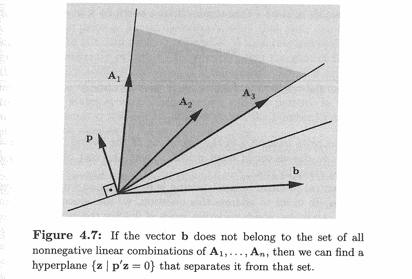
当 \(b\) 不落在 \(A_i\) 和 \(x \geq 0\) 构造出的阴影范围内，也就是说第一个条件不满足的时候，就一定存在 \(p\) 使得 \(p\) 和 \(b\) 的夹角是“钝角”，而且 \(p\) 和每个 \(A_i\) 的夹角是“锐角”。

考虑一个有 \(n\) 种商品的贸易过程，每次购买的份额是一个 asset vector \(x = (x_1,x_2,...,x_n)\)，初始状态下的价格是一个 price vector \(p = (p_1,p_2,...,p_n)\)，因此初始状态下投入的资金是 \(p^Tx\)。一段时间后会呈现出 \(m\) 种状态之一，第 \(i\) 种状态下这 \(n\) 种商品的售价是一个 payoff vector \((r_{i1},r_{i2},...,r_{in})\)。由此构造一个 payoff matrix：

\[R= \begin{bmatrix} r_{11} & r_{12} & \cdots & r_{1n} \\ \cdots & \cdots & \cdots & \cdots \\\cdots & \cdots & \cdots & \cdots \\ r_{m1} & r_{m2} & \cdots & r_{mn} \end{bmatrix}\]

取 \(w = Rx = (w_1,w_2,\cdots,w_m)\) 作为购买份额为 \(x\) 时，最终在 \(m\) 个状态下分别得到的收入。有一个 absence of arbitrage condition，大概就是说不可能在负投资的状态下得到正收益，也就是说 \(Rx \geq 0\) 可以推出 \(p^Tx \geq 0\)。

由 Farka's lemma 可知此时第二条不成立，一定存在 \(q \geq 0\) 使得 \(R ^T q = p\)。

The Center of Gravity Method

实际上就是一个不断切割已有的 polyhedron 来找到 optimal solution 的过程。简单来说从初始状态开始，每个状态下手里有一个多边形 \(S_t\)（feasible set 的 subset）和它的质心 \(x_t\)，然后把使得取值大于 \(c^Tx_t\) 的部分切掉，也就是取 \(S_t\) 和 hyperapce \(\{x \in \mathbb R^n \mid c^T(x-x^T) > 0 \}\) 的交这一部分作为不可能取到 optimal cost 的区域，余下的部分是下一状态的多边形 \(S_{t+1}\) 和相应的质心 \(x_{t+1}\)，由此按照所需的精度来逼近 optimal cost。

写成算法的步骤来说也非常简单，实际上每次就操作两步。先取整个 feasible set 作为 \(S_1\)，然后：

1. Take \(x_t = \frac{1}{Vol(S_t)} \int_{x \in S_t} x \; dx\) as the center of gravity of the polyhedron \(S_t\);
2. Take \(S_{t+1} = S_t \cap \{x \mid c^T(x-x_t) \leq 0 \}\) as the new polyhedron.

一直重复直到 \(S_t\) 足够小，此时 \(c^T x_t\) 和 optimal cost \(c^Tx^*\) 的误差也会足够小。这由一些定理保证。

• Let \(K\) be a centered convex set (i.e. \(\int_{x \in K} xdx=0\)), then for any \(w \in \mathbb R^n\), \(w \neq 0\), one has

  \[Vol(\mathcal K \cap \{x \in \mathbb R^n : x^T w \geq 0\}) \geq \frac 1 e Vol(\mathcal K)\]

这告诉我们每个新的多边形和原多边形之间有一个体积关系是 \(Vol(S_{t+1}) \leq (1-\frac 1 e) Vol(S_t) \leq \cdots \leq (1-\frac 1 e)^t Vol(S_1)\)，再对于 \(\varepsilon = (1-\frac 1 e)^{t/n}\) 取 \(\mathcal S_\varepsilon = \{(1-\varepsilon )x^* + \varepsilon x, \forall x \in S_1\}\)，实际上是对 \(S_1\) 做了一个仿射变换。此时有 \(Vol(S_\varepsilon)=\varepsilon^n Vol(S_1) = (1-\frac 1 e)^tVol(S_1) \geq Vol(S_{t+1})\)，于是可以找到一个 \(x_\varepsilon \in S_\varepsilon\) 使其在 \(t\) 时刻时仍在 \(S_t\) 中，而 \(t+1\) 时刻就被“裁剪”了出去。

所以有

\[c^Tx_{t+1} < c^Tx_\varepsilon = c^T((1-\varepsilon)x^*+ \varepsilon x) \leq c^Tx^* + 2B\varepsilon =c^Tx^*+2B(1-\frac 1 e)^{t/n}\]

也就是说 \(c^Tx_{t+1} - c^Tx^* < 2B(1-\frac 1 e)^{t/n}\) 作为 \(t+1\) 时刻下取值距离 optimal cost 的误差可以被控制，并且我们可以在 \(O(n \log(\frac{1}{\varepsilon}))\) 时间下得到误差为 \(\varepsilon\) 的 cost 和 solution。这比 simplex method 误差大一些，但是 polynomial time algorithm。

The Ellipsoid Method

讲这个的时候我太困了，上楼找了个教室睡觉，没听。我估计我困成那样听也听不懂，他这个手稿太抽象了也看不大懂，貌似书上也没这一部分，哥们有点子崩溃（。等 scribing 了。

我都学会了 scribing 还没出来，自己写一个吧。

Notations

首先是一些记号：

• A set \(E\) of vectors in \(\mathbb R^N\) of the form \(E = E(z,D) = \{x \in \mathbb R^n \mid (x- z)^T D^{-1} (x-z) \leq1 \}\), where \(D\) is an \(n \times n\) positive definite symmetric matrix, is called an ellipsoid with center \(z \in \mathbb R^n\).

• If \(D\) is a \(n \times n\) nonsingular matrix and \(b \in \mathbb R^n\), then the mapping \(S: \mathbb R^n \to \mathbb R^n\) defined by \(S(x) = Dx + b\), is called an affine transformation.

注意到仿射变换都是可逆的，所以可以把仿射变换的像定义成

• \(S(L) = \{y \in \mathbb R^n \mid y = Dx +b, \text{for some } x\in L \}\)
• The volume of a set \(L \in \mathbb R^n\), which is denoted by \(Vol(L)\), is defined as \(Vol(L) = \int_{x \in L}dx\)

然后就可以得到仿射变换后的体积是

• If \(S(x) = Dx + b\) then \(Vol(S(L)) = |det(D)| Vol(L)\)

  Proof: \(Vol(S(L)) = \int_{y \in S(L)} dy = \int_{x \in L} |det(D)| dx = |det(D)| Vol(L)\)

Algorithm

目标是考虑一个 \(Ax \geq b\) 形式的优化问题的 feasible set，也就是一个 polyhedron \(P\) 是否是空集的问题，可以用一个 Ellipsoid Algorithm 来解决。既然是用迭代算法解决，其实就不能太苛求精细程度，我们约定最后得到的覆盖椭圆的面积小于 \(\varepsilon\) 时就认为 \(P\) 是一个空集。

首先考虑一个覆盖所求 polyhedron \(P\) 的椭圆 \(E_t\)，如果其中心 \(x_t \in P\) 则找到了一个 \(P\) 中的解，可以得出 \(P\) 是非空的；如果 \(x_t \notin P\) 那么 \(x_t\) 一定违反了其中的某个 constraint \(a_i ^Tx \geq b_i\)，\(P\) 一定在 halfspace \(\{x \in \mathbb R^n \mid a_i^T x \geq a_i^Tx_t \}\) 和 \(E_t\) 的交集里，这样我们再做一个新的更小的椭圆 \(E_{t+1}\) 来覆盖这一部分，就可以继续这一算法。

来个我非常喜欢的图！

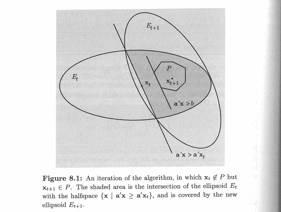
现在需要解决的问题仍然是 termination 问题，也就是是否 \(E_{t+1}\) 的体积一定比 \(E_t\) 更小。以下定理保证了它们的体积之间一定有一个指数级的减少：

• Let \(E = E(z,D)\) be an ellipsoid in \(\mathbb R^n\), and let \(a\) be a nonzero vector. Consider the halfspace \(H = \{x \in \mathbb R ^n \mid a^Tx \geq a^T z \}\) and let

  \[\bar z = z + \frac{1}{n+1} \frac{Da}{\sqrt{a^TDa}}\]

  \[\bar D = \frac{n^2}{n^2-1} (D - \frac{2}{n+1} \frac{Daa^TD}{a^TDa})\]

  Then \(\bar D\) is positive definite and the new ellipsoid \(\bar E = E(\bar z, \bar D)\) satisfies the following properties:

  • \(E \cap H \subset \bar E\)
  • \(Vol(\bar E) < e^{-1/(2(n+1))} Vol(E)\)

  Proof: First consider \(a = e_1. D = I_{n \times n}\) and the center of \(E_0\) as \(z = 0\). It's trivial to see that the first property holds. In this case the positive definite matrix of \(\bar E_0\) is \(D = diag((\frac{n}{n+1})^2, \frac{n^2}{n^2-1}, \cdots,\frac{n^2}{n^2-1})\), and the center is \(a = (\frac{1}{n+1},0,\cdots,0)^T\).

  Now by constructing an affine transformation we can consider the general case. The transformation T should let \(T(E) = E_0, T(H) = H_0\) and \(T(\bar E) = \bar E_0\). By some elementary observations we can obtain that affine transformations preserve set inclusion, i.e. if \(E_0 \cap H_0 \subset \bar E_0\), then there is \(T(E_0) \cap T(H_0) \subset T(\bar E_0)\), therefore the first property holds naturally.

  Let \(R\) be the rotation matrix corresponding to the vector \(u = D^{\frac 1 2} a\), i.e.,

  \[R^TR = I, \quad RD^{\frac 1 2}a_i = \|D^{\frac 1 2} a_i \| e_1\]

  Consider the following affine transformation:

  \[T(x) = R(D^{-\frac 1 2}(x-z))\]

  Therefore,

  \(\begin{aligned} x \in E & \iff (x-z)^TD^{-1}(x-z)\leq 1 \\ & \iff (x-z)^TD^{-\frac 1 2}R^TRD^{-\frac 1 2}(x-z)\leq 1 \\ & \iff T(x)^T T(x) \leq 1 \\ & \iff T(x) \in E_0, \end{aligned}\)

  which implies that \(T(E) = E_0\).

  Similarly,

  \[\begin{aligned} x \in H & \iff a_i^T(x-z )\geq 0 \\ & \iff \|D^{-\frac 1 2}a_i \| e_1 ^T RD^{-\frac 1 2} (x-z) \geq 0 \\ & \iff e_1 ^T T(x) \geq 0 \\ & \iff T(x) \in H_0, \end{aligned}\]

  which implies \(T(H) = H_0\).

  Moreover there is also \(T(\bar E) = \bar E_0\) and we omit the complicated algebraic manipulations. Therefore \(E \cap H \subset \bar E\) holds according to the properties of affine transformation. Next we prove the conclusion about the volume.

  \(\frac{Vol(\bar E)}{Vol(E)} = \frac{Vol(T(\bar E))}{Vol(T(E))} = \frac{Vol(\bar E_0)}{Vol(E_0)} = det(D_0 ^{\frac 1 2}) = (\frac{n}{\sqrt{n^2-1}})^{n-1}(\frac{n}{n+1})\)

  Consider

  \[(\frac{n^2}{n^2-1})^{\frac{n-1}{2}}(\frac{n}{n+1}) = (1+\frac{1}{n^2-1})^{\frac{n-1}{2}}(1-\frac{1}{n+1}) \leq (e^{\frac{1}{n^2-1}})^{\frac{n-1}{2}} e^{-\frac{1}{n+1}} = e^{-\frac{1}{2(n+1)}},\]

  and the desired result follows.

另外如果估计得再精细一点的话下界其实是 \(\exp(-\frac{1}{2n})\)（详见 Bubeck），可以对函数求导做。

所以只要初始状态的 ellipsoid 体积有限，算法一定会在有限时间内终止，可以用来解决 feasiblility 的问题，这是一个可以在 \(O(n \log \varepsilon)\) 时间内结束的算法，实际上对于找 feasible solution 来说还是很快的。但 feasible solution 一个单点对于优化问题来说其实没什么用，我们的目标仍然是寻找 optimal cost，为此需要一些类似于 center of gravity method 的方法。

另外 ellipsoid method 也可以用来解决 optimal cost 的逼近，有这样一个体积关系了之后原理和 center of gravity method 类似：

每个新的 ellipsoid 和上一时刻 ellipsoid 之间有一个体积关系是 \(Vol(S_{t+1}) \leq \exp(-\frac{1}{2n}) Vol(S_t) \leq \cdots \leq \exp(-\frac{t}{2n}) Vol(S_1)\)，再对于 \(\varepsilon = \exp(-\frac{t}{2n^2})\) 取 \(\mathcal S_\varepsilon = \{(1-\varepsilon )x^* + \varepsilon x, \forall x \in S_1\}\)，实际上是对 \(S_1\) 做了一个仿射变换。此时有 \(Vol(S_\varepsilon)=\varepsilon^n Vol(S_1) = \exp(-\frac{t}{2n}) Vol(S_1) \geq Vol(S_{t+1})\)，于是可以找到一个 \(x_\varepsilon \in S_\varepsilon\) 使其在 \(t\) 时刻时仍在 \(S_t\) 中，而 \(t+1\) 时刻就被“裁剪”了出去。

所以有：

\[c^Tx_{t+1} < c^Tx_\varepsilon = c^T((1-\varepsilon)x^*+ \varepsilon x) \leq c^Tx^* + 2B\varepsilon =c^Tx^*+2B \exp(-\frac{t}{2n^2}),\]

也就是说 \(c^Tx_{t+1} - c^Tx^* < 2B \exp(-\frac{t}{2n^2})\) 作为 \(t+1\) 时刻下取值距离 optimal cost 的误差可以被控制，并且我们可以在 \(O(n^2 \log(\frac{1}{\varepsilon}))\) 时间下得到误差为 \(\varepsilon\) 的 cost 和 solution。同样是得到的 cost 比 simplex method 误差大一些并非精确值，但是 polynomial time algorithm，虽然比起 center of gravity method 来说消耗更大，但也有它的优势。

之前的想法一直有大问题，我当时也没怎么看懂 Bubeck 那本书的内容，更是完全不理解为什么 time usage 里面还有 \(R/r\) 的项。今晚做出来优化作业第一题之后醍醐灌顶，直接复制到这里来就很清楚了。

Problem: Consider the following convex optimization problem (\(f,g_i\) are convex):

\[\text{minimize} \quad f(x)\]

\[\text{subject to} \quad g_i(x) \leq 0, i=1,2,\cdots,m.\]

Let \(\mathcal K = \{x \mid g_i(x) \leq 0, i=1,2,\cdots,m\}\). Assume that there exists \(x_,x_0^\prime\) s.t. \(\mathcal K\) is between balls of radius \(r,R\),

\[B(x_0,r) \subseteq \mathcal K \subseteq B(x_0^\prime,R)\]

Further assume that \(\sup_{x \in \mathcal K} |f(x)| \leq B\). Given any \(x \in \mathbb R^n\) one can evaluate \(f(x),g_i(x), \nabla f(x) , \nabla g_i(x)\). Propose an efficient implementation of the Ellipsoid's method. Prove that the algorithm converges in \(\mathcal O(n^2 \log(\frac{BR}{r \varepsilon}))\) iterations to find an \(\varepsilon\) optimal solution.

Solution: To begin the algorithm, we set \(\mathcal E_0 = B(x_0^\prime, R)\) and \(c_0 = x_0^\prime\) as its center. At time \(t\) we divide the possible results into two situations as follows.

• If \(c_t \notin \mathcal K\), then there is some constraints \(g_i(x) \leq 0\) violated so that \(c_t\) does not lie in the feasible set. We find the violated constraints by calling the zeroth order oracle \(g_i(c_t)\) and compare their value with \(0\). To save the computational source we just pick the violated constraint \(g_i(c_t) >0\) with the smallest subscript, and number it as \(g_i^{(t)}\).

  Thus the feasible set \(\mathcal K\) lies in \(\mathcal E _t \cap \{x \mid g_i ^{(t)} (x) \leq g_i ^{(t)} (c_t)\} \subseteq \mathcal E _t \cap \{x \mid \nabla g_i^{(t)}(c_t)^T (x-c_t) \leq 0\}\) according to the definition of subgradient. And the exact value of subgradient \(\nabla g_i^{(t)}(c_t)\) can be obtained by calling the first order oracle \(\nabla g_i^{(t)}\).

  Then we can just construct the \((t+1)\)-th ellipsoid by covering the set shown above, i.e. \(\mathcal E_{t+1} \supseteq \mathcal E _t \cap \{x \mid \nabla g_i^{(t)}(c_t)^T (x-c_t) \leq 0\}\).

• The second case is much easier. If we found \(c_t \in \mathcal K\), by considering the subset \(\mathcal E_t \cap \{ x \mid f(x) < f(c_t)\} \subseteq \mathcal E_t\), we can either find \(c_t\) is optimal by observing that the set is empty or found a better solution through iteration.

  According to the definition of subgradient, there is \(\mathcal E_t \cap \{x \mid f(x) < f(c_t)\} \subseteq \mathcal E_t \cap \{ x \mid \nabla f(c_t)^T (x-c_t) \leq 0\}\). Then we can just construct the \((t+1)\)-th ellipsoid by covering the set shown above, i.e. \(\mathcal E_{t+1} \supseteq \mathcal E _t \cap \{ x \mid \nabla f(c_t)^T (x-c_t) \leq 0\}\), in which the value of subgradient \(\nabla f(c_t)\) can be obtained by calling the first order oracle \(\nabla f\).

For both situations, we can obtain \(\mathcal E_{t+1}\) with the least volume such that \(Vol(\mathcal E_{t+1} ) \leq \exp(-\frac{1}{2n}) Vol(\mathcal E_t)\) according to the theorem we proved in class (and we can construct the exact form of \(\mathcal E_{t+1}\) through the complex equation, which won't be shown again in this solution).

Therefore, if \(t \geq 2n^2 \log(\frac{R}{r})\) there is \(Vol(\mathcal E_t) \leq Vol(B(x_0,r))\) and \(\{c_1,c_2,\cdots,c_t\} \cap \mathcal K \neq \varnothing\). From now on we only consider the time that ensures \(\{c_1,c_2,\cdots,c_t\} \cap \mathcal K \neq \varnothing\).

For fixed \(\varepsilon >0\), we take \(\mathcal K_\varepsilon = \{(1-\varepsilon)x^* + \varepsilon x \mid \forall x \in B(x_0,r)\}\) as an affine transformation, in which \(x^*\) is the optimal solution of this problem. Moreover we denote \(x_t \triangleq \arg \min_{c_s \in \{c_0,c_1,\cdots, c_t\} \cap \mathcal K} f(c_s)\).

When we take \(\varepsilon = \frac{R}{r} \exp(-\frac{t}{2n^2})\) there is \[Vol(\mathcal K_\varepsilon ) = \varepsilon^n Vol(B(x_0,r)) = \varepsilon^n (\frac{r}{R})^n Vol(B(x_0^\prime ,R)) = \exp(-\frac{t}{2n^2}) Vol(B(x_0^\prime, R)) > Vol(\mathcal E_t)\]

This inequality implies that there exists one time \(r \in \{1,2,\cdots,t\}\) s.t. there exists \(x_\varepsilon \in \mathcal K_\varepsilon\), \(x_\varepsilon \in \mathcal E_{r-1}\), but \(x_\varepsilon \notin \mathcal E_r\), therefore \(x_\varepsilon\) is not optimal. According to the convexity of \(f(x)\), there is \[f(x_t) < f(c_r) \leq f(x_\varepsilon) = f((1-\varepsilon)x^* + \varepsilon x_r) \leq (1-\varepsilon) f(x^*) + \varepsilon f(x_r) \leq f(x^*) + 2B\varepsilon,\] which implies that \[f(x_t) - f(x^*) \leq 2B\varepsilon = \frac{2BR}{r} \exp(-\frac{t}{2n^2}).\]

Then we can conclude that the algorithm converges in \(\mathcal O(n^2 \log(\frac{BR}{\varepsilon r}))\) iterations to find an \(\varepsilon\) optimal solution, and the desired result follows.

Lecture 4

睡了（，等个笔记（（

10.23 UPD：今天布置了个优化 HW3 但又迅速删掉了，我也不知道为什么要同时把讲义也删掉，当时正好在贴所以也没来得及下（。这助教是否也是一个优化算法控制的，要传就把所有的东西都传上来要删就全部删掉，来保证要么所有人都满意要么所有人都不满意（。

Convex Optimization

Notations

#每日迷神

• A set \(C \in \mathbb R^n\) is affine iff for any \(x,y \in C\) and any \(\theta \in \mathbb R\), there is \(\theta x + (1-\theta) y \in C\), therefore the whole line lies in \(C\).
  • Therefore, if \(C\) is an affine set and \(x_0 \in C\), then the set \(V = \{x-x_0 \mid \forall x \in C\}\) is a subspace.
• An affine hull of \(C\) is denoted as \(aff(C) = \{\theta_1 x_1+ \theta_2 x_2+\cdots+ \theta_k x_k \mid \forall k \in \mathbb Z_+, x_i \in C, \theta_i \in \mathbb R \}\)
• The relative interior \(relint(C) = \{x\in C \mid \exist r >0 , \text{s.t. } B(x,r) \cap aff(C) \subseteq C \}\)

简单来说，affine set/affine hull 和 convex 版本的唯一区别就是参数不需要取在 \([0,1]\) 之间，所以它一般是个平面。

• A set \(C\) is called a cone iff \(\forall x \in C\) and for any \(\theta > 0\), there is \(\theta x \in C\).

• (Extended convex function) A function \(f : \mathbb R^n \to \mathbb R\) is convex, we can extend its domain \(dom(f)\) to \(\mathbb R^n\) by taking \(f(x) = \infty\) for any \(x \notin dom(f)\).

• (Epigraph of a function) \(epi(f) = \{(x,t) \mid t \geq f(x)\}\)

  Therefore \(f\) is a convex function if and only if \(epi(f)\) is a convex set.

Basic Theorems

• (Seperating Hyperplane Theorem) Suppose \(C,D\) are nonempty disjoint convex sets, then there exists \(a \neq 0\), \(a,b \in \mathbb R^n\) s.t. \(C \subseteq \{x \in \mathbb R^n \mid a^Tx \leq b\}\) and \(D \subseteq \{x \in \mathbb R^n \mid a^Tx \geq b\}\).

  Proof: We only consider the case when \(C,D\) are both closed and bounded.

  Define \(dist(C,D) = \inf\{\|u-v\|_2 \mid u \in C,v \in D \}\) as the distance between \(C,D\), then by closed and boundness we can find \(c \in C, d \in D\) s.t. \(dist(C,D) = \|c-d\|_2\). Take \(a = d-c\), \(b = \frac 1 2 (\|d\|_2^2 - \|c\|_2^2)\).

  Then the affine transformation \(f(x) = a^Tx - b\) will let \(f(x) <0\) for any \(x \in D\), and \(f(x) >0\) for any \(x \in C\).

• (Supporting Hyperplane Theorem) Suppose \(C\) is convex, then for any \(x \in bd(C)\) here exists a supporting vector \(a \neq 0, a \in \mathbb R^n\), s.t. \(\forall x \in C\), \(a^Tx_0 \leq a^Tx\). (\(bd(C)\) is the boundary of \(C\))

别的没什么了，convex function 的性质什么的真没必要再写一遍了，他又不讲 subgradient。

Lecture 5

才隔了两周，今天怎么又是哥们在做 scribing 啊（。read-only 的链接在这里。

今天讲一些 convex optimization 里的例子，给哥们整的一愣一愣的。

Examples in Convex Optimization

Notations

#每日迷神

你还别说现在还真不一定书上都有了，那个 max cut 给哥们整不会了，Boyd 上面没写，Bubeck 就写了一点而且还把课上的内容跳过去了。而且 Bubeck 本来就简略，看了个寂寞。

• The following optimization problem is called a convex optimization problem if \(x_0, f_i\) are convex, and \(h_i\) are linear:

  \[\begin{aligned} \textbf{minimize} \quad & f_0(x) \\ \textbf{subject to} \quad & f_i(x) \leq 0 \\ & h_i (x) =0 \end{aligned}\]

• \(x\) is a \(\varepsilon\)-suboptimal if \(f_0(x) \leq p^* + \varepsilon\), in which \(p^*\) is the optimal value of the convex optimization problem.

• \(x_0\) is locally optimal if there exists \(R >0\) s.t. \(x_0\) is the optimal solution to:

​ \[\begin{aligned} \textbf{minimize} \quad & f_0(x) \\ \textbf{subject to} \quad & f_i(x) \leq 0 \\ & h_i (x) =0 \\ & \|x-x_0\| \leq R \end{aligned}\]

Why Convex Optimization?

为什么研究凸优化？一个是 linear programming problem 有它的局限性，许多问题只能往凸优化的方向转化。另外凸性质实际上是非常美妙的。下面是一个很 trivial 的例子，我们对 convex optimization 的转化问题的探究远不止于此。

Why is convex optimization important? That's because some non-convex problems have underlying convexity. For example, we consider the following optimization problem:

\[\begin{aligned} \textbf{minimize} \quad & f_0(x)=x_1^2+x_2^2 \\ \textbf{subject to} \quad & f_1(x) = \frac{x_1}{1+x_2^2} \leq 0 \\ & h_i (x) = (x_1+x_2)^2 =0 \end{aligned}\]

which can easily be transformed into a standard convex optimization problem.

Example: Max Cut Problem

别 TCS 了求你了求你了求你了（

通过一个 max cut problem 来体现从 nonconvex optimization 向 convex optimization 的转化，从方法论的层面上来说是两步。

Why are convex optimization problems important? That's because many non-convex optimization problems can be transformed into convex ones, and we can solve convex optimization problems through mature technologies. Generally speaking, the process contains two steps:

1. First, transform the non-convex problem into convex ones through relaxation.
2. Next recover a solution from the convex problem to the non-convex one through random rounding.

Notations

• A cut in an undirected graph \(G = (V, \mathcal E)\) is defined as \(A \subseteq V\).The capacity of a cut \(A\) is defined as \(c(A) = | \{(u,v)\in \mathcal E \mid u \in A, u \in A^c\}|\).

而 max cut 问题就是寻找最大的 \(c(A)\)，尽管我不知道这样做有什么意义，但它是 NP-hard 的。所以我们只需要找到一个 polynomial time 的算法就可以证明...（逃

• ​ An \(\alpha\)-approximate max cut is a cut \(A\) s.t. \(c(A) \geq \alpha \max_{U \subseteq V} c(U)\).

\(\frac 1 2\)-Approximate Approach

怎么是概率做法，真稀奇。

To be more specific, we can give a \(\frac{1}{2}\)-approximate max cut by randomly adding each point \(v\) in \(V\) to the cut \(A\) with probability \(\frac{1}{2}\). Consider the expectation of \(c(A)\) here and we can get:

\[\mathbb E_A(c(A)) = \mathbb E_A \sum_{(u,v)\in \mathcal E} 1_{(u \in A,v \in A^c)} = \sum_{(u,v) \in \mathcal E} P(u \in A, v \in A^c) = \sum_{(u,v) \in \mathcal E} \frac{1}{2} = \frac{|\mathcal E|}{2}.\]

然而这还是很粗糙。

Linear Approach

如果没有 convex optimization 的话就是考虑一些 linear programming 的近似，举两个失败的 approach 说明这很困难：

• Consider the following formulation of the problem:

  \[\begin{aligned} \textbf{maximize}_{x\in \mathbb R^n} \quad & \sum_{(u,v)\in \mathcal E} \frac{1}{2}(1-x_ux_v) \\ \textbf{subject to} \quad & x_v \in \{-1,1\} \end{aligned}\]

• This is not a linear programming problem, and we can transform it by denoting \(z_e = x_ux_v, e=(u,v) \in \mathcal{E}\):

  \[\begin{aligned} \textbf{maximize}_{x,z} \quad & \sum_{e \in E} \frac{1}{2 } (1-z_e) \\ \textbf{subject to} \quad & z_{(u,v)} \geq -x_u -x_v -1 \\ & z_{(u,v)} \geq x_u +x_v -1 \\ & x_v \in [-1,1] \end{aligned}\]

However, this still fails for we can choose \(x_v =x_u=0\) and \(z_{(u,v)} =-1\) in the feasible set, which means the approach will only give a randomized choice of \(A\). Now turn to convex optimization for help.

Convex Transformation

• The basic idea is to replace \(x_u.x_v\) with \(n-1\) dimensional vectors and construct an auxiliary problem, which is called semi-definite relaxation:

  \[\begin{aligned} \textbf{maximize} \quad & \sum_{(u,v) \in \mathcal E} \frac{1}{2} (1-x_u^Tx_v) \\ \textbf{subject to} \quad & x_u \in S^{n-1} \text{ for any }u=1,2,\cdots,n \end{aligned}\]

  in which \(S^{n-1}\) is the unit sphere in \(\mathbb R^{n-1}\). Observe that \(\frac{1}{4}\|x_u-x_v\|^2 =\frac{1}{4} (x_u -x_v)^T(x_u-x_v) = \frac{1}{2} (1-x_ux_v)\), and \(\frac{1}{2} \sum_{e \in \mathcal E} (1-z_e) = \frac{1}{4} \sum_{(u,v)\in \mathcal E} \|x_u - x_v\|^2\).

  Now we take \(\text{Maxcut}^\circ (C)\) as the optimal cost of the auxiliary problem and denote \(\text{Maxcut} (C)\) as the optimal cost of the original problem. Then there is \(\text{Maxcut} (C) \leq \text{Maxcut}^\circ (C)\) because any optimal solution of the original problem can be transformed into a feasible solution in the auxiliary one.

  To be more precise, if \(\{x_u\}\) is an optimal solution to the original problem, then for any \(x_u = 1\) there is \(x_v = -1\) for each \(v \in \{v \mid (u,v) \in \mathcal E\}\). Therefore we can take \(x_u = e_1\), \(x_v = -e_1\) for any \(v \in \{v \mid (u,v) \in \mathcal E\}\) as a feasible solution to the auxiliary problem, and the cost is equal to the optimal cost of the original one.

• However the auxiliary problem is still non-convex, we'd like to consider another optimization problem as follows:

  \[\begin{aligned} \textbf{minimize} \quad & X \cdot A = \sum_{i,j \in V} X_{ij} A_{ij} \\ \textbf{subject to} \quad & X \geq 0 \; \\ & X_{ii}=1 \end{aligned}\]

  in which \(X \geq 0\) means \(X\) is semi-definite, i.e. \(X \in S_+^n, X \in \mathbb R^{n \times n}\).

  We set \(A_{ij}=1\) if \((i,j) \in \mathcal E\), else \(A_{ij}=0\). Now we prove that the two problems above are equivalent.

• The following two max-cut optimization problems are equivalent:

​ \[\begin{aligned} ​ \textbf{maximize} \quad & \sum_{(u,v) \in \mathcal E} \frac{1}{2} (1-x_u^Tx_v) \\ ​ \textbf{subject to} \quad & x_u \in S^{n-1} \\ ​ \\ ​ \end{aligned} \quad \quad \quad ​ \begin{aligned} ​ \textbf{minimize} \quad & X \cdot A = \sum_{i,j \in V} X_{ij} A_{ij} \\ ​ \textbf{subject to} \quad & X \geq 0 \; \\ ​ & X_{ii}=1 ​ \end{aligned}\]

Proof: Note that \(X_{ij} = x_i^T x_j\) (and sometimes \(X\) is called the gram matrix), therefore

\[\begin{aligned} X \in S_+^n \text{ is feasible } & \iff X_{ij}=1 \text{ for any } i \in V \\ & \iff \|x_u \|=1 \text{ for any } u \in V \\ & \iff x_u \in S^{n-1} \text{ for any } u \in V \end{aligned}\]

and the desired result follows.