数理统计初探——统计推断

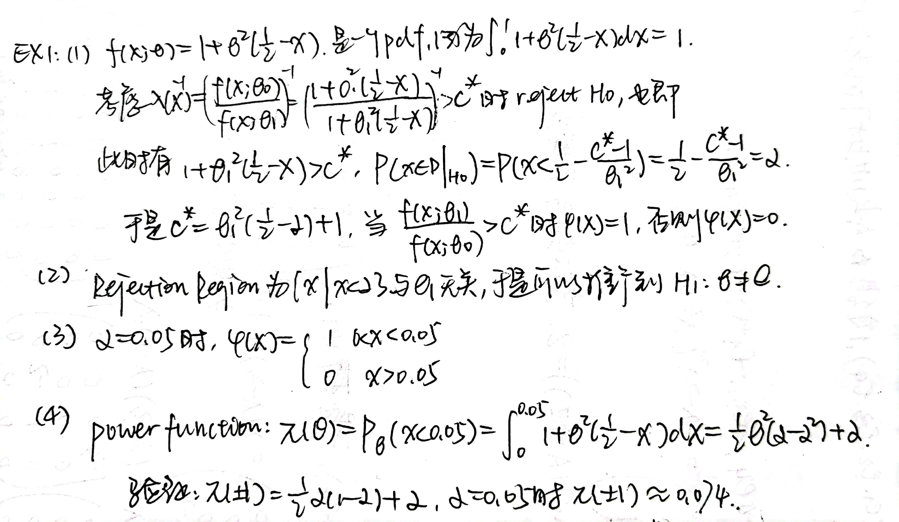
据说统计推断是统辅基础五大件里最难的，这门课也可以直接称为数理统计（基础）。我初概的体验并不是很好，甩锅给了不匹配的教材，还记了 PF。但统计推断要洗心革面好好上，也打算做预习。不仅是因为不打算再去数学系回炉重造，也是担心留下一种隐隐怀疑自己并不是很适合学统计的感觉，本科过半又换方向的试错成本就略高了。

不过，我确实也很好奇到底适不适合、有多感兴趣呢？真不行的话，该换还得换呀。

这课的 PPT 是英文，老师讲课用中文，教材英文中译都有，图书馆借来的是中文版，据说考试卷子是英文的。

妈呀.jpg，所以以下遇到名词的话会中英都写。一些懒得打的东西就直接通过截图 PPT 或者手写拍照给出，主要我也怕我把写的东西弄丢了（。

Lecture 1

先吹了会水，尽管课时紧张，还是要骗骗大家统计学前景非常广阔 x

本节介绍统计推断中的一些基本概念，对应教材第五章《随机样本的性质》。

研究范围约定及基本定义

• 研究范围的约定：在研究大量数据、确定其行为时，因为难以全部分析，我们会对其进行多次随机抽样（Sampling），研究多次得到的样本的性质，以及“多次”中蕴含的性质，来推断总体数据的性质。这是统计推断的核心思想之一。以下约定一些术语。

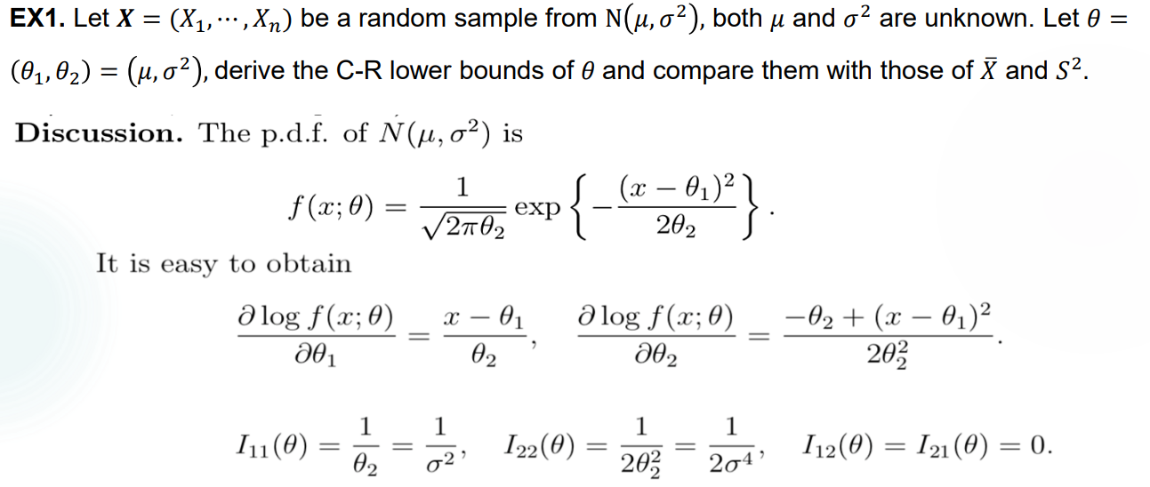
  • Population（总体）：总的研究范围，用一个随机变量 \(X\) 来概括，\(X\) 服从有某些参数 \(\theta\) 的分布 \(F\)。我们的目标正是通过抽样来找到这个分布 \(F\)，从而刻画 Population 的性质。

  • Population parameters：用于表征 Population 的性质，比如期望，方差，矩，也就是上述的 \(\theta\)。例如，对于一个服从正态分布的 Population，它的 Population parameters 记为 \(\theta=(\mu, \sigma^2)\)。

  • Sample（样本）：多次抽样得到的随机变量 \(X_1,X_2,...,X_n\) 独立同分布，有相同的（边缘）概率密度函数（PMF） \(f(x)\)，则称其为 Population 中的（随机）样本。

  • Sample size（样本量）：显然上述的那个 \(n\) 就是样本量，表征样本大小，trivial。

  举个例子。现在有 10000 个产品，其中有一部分废品。我们想知道大约有多少废品又不希望检测所有的产品，于是每次抽样 100 个进行检测。此处的 Population 就是指 10000 个产品，每次的 Sample 是抽到的 100 个样品，Sample size 是100。可以在 Population 上定义随机变量 \(X\)，如果产品是废品则 \(X=1\)，合格则 \(X=0\)，则每个样本可以表征为 \(X=\lbrace X_1,X_2,...,X_n\rbrace\)。

  在我们抽样之前，\(X_i\) 都还是未知的随机变量，和 Population 同分布。然而抽样之后，\(X=\lbrace X_1,X_2,...,X_n\rbrace\) 就成为了一个确切的，由实数组成的数组，比如在上述例子中，某次抽样得到的结果是一个由 \(0,1\) 表示的数组。

  • Sample space（样本空间）：和概率论中的样本空间不太一样的是，这里的样本空间表示所有抽样可以得到的数组，用 \(\chi\) 表示，这个符号和 Chi-Square 分布的符号是相同的。在上述例子中，就是：\(\chi = \lbrace (x_1,x_2,...,x_{100}) | x_i \in \lbrace 0,1 \rbrace,i=1,2,...,100\rbrace\)。

  • Simple random sampling：怎么定义随机抽样？如果能使得到的 \(X_1,X_2,...,X_n\) 独立同分布（\(i.i.d. \sim F\)），那么这种抽样方式就是简单随机抽样，也称为随机抽样。

    需要注意的是，简单随机抽样是有放回的，否则抽到某一元素的概率会不断变化，并不是独立的。

  • Joint distribution function：\(F(x_1,x_2,...,x_n)=F(x_1)F(x_2)...F(x_n)\)

  • Joint density function (if exists)：\(f(x_1,x_2,...,x_n)=f(x_1)f(x_2)...f(x_n)\)

统计量

• 定义了这么多东西之后，我们可以研究抽取出来的随机样本 \(X_1,X_2,...,X_n\)，研究方式是定义一些关于这些随机样本的函数，研究函数的性质。

  • Statistic（统计量）：记抽取得到的随机样本 / 数据为 \(X_1,X_2,...,X_n\)，函数 \(T(X_1,...,X_n)\) 称为一个统计量。显然，在抽取之前它是一个随机变量的函数，也即一个随机向量；但在抽取之后，\(T\) 可以计算为一个实数。

    作为随机变量，\(T\) 的概率分布称为 Sampling Distribution，抽样分布。

  • 亿些常用的 Statistic：

    Sample mean：\(X = \frac{1}{n} \Sigma_{i=1}^n X_i\)

    Sample variance：\(S^2 = \frac{1}{n-1} \Sigma_{i=1}^{n} (X_i-X) ^2\)

    Sample standard deviation：\(S\)

    K-th origin moment（k 阶矩）：\(a_{n,k} = \frac{1}{n} \Sigma _{i=1} ^{n} X_i ^k, k =1,2,...\)

    K-th center moment（k 阶中心矩）：\(m_{n,k} = \frac{1}{n} \Sigma _{i=1} ^{n} (X_i-X) ^k, k =2,3,...\)

    Order statistic（次序统计量）：排列所有的样本为 \(X_ {(1)} \leq X_ {(2)} \leq ... \leq X_{(n)}\)，则 \((X _{(1)}, X _{(2)},...,X _{(n)})\) 是次序统计量。

    Sample medium（中位数）：\(m_{\frac{1}{2}}=X_{n/2}\) 或者 \(\frac{1}{2} (X _{n/2}+X _{n/2+1})\)

    Extremum of sample：\(X _{(1)},X _{(n)}\)

    Sample p-fractile（\(0<p<1\)）：\(m_p = X_{(m)}\)，其中 \(m=[(n+1)p]\)

    Sample range（极差）：\(R=X _{(n)}-X _{(1)}\)

    Sample coefficient of variation（样本变异系数）：\(v=\frac{S}{X}\)

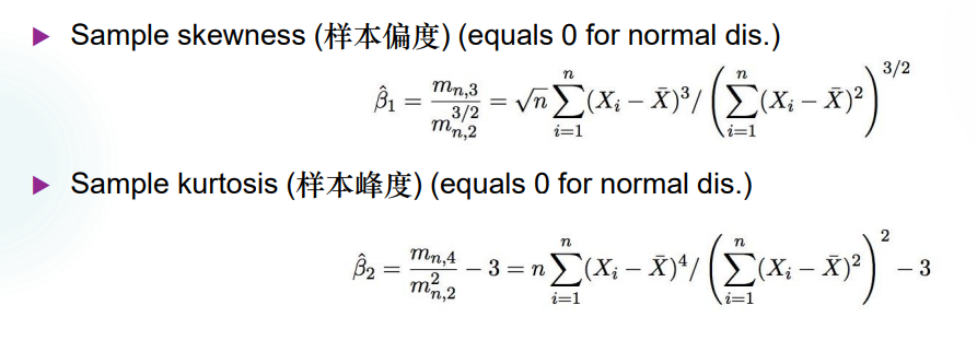
    Sample skewness（样本偏度），Sample kurtosis（样本峰度）自查：

    

    Empirical distribution function（经验分布函数）：

    \(I_A(x)=1 \\; for \\; x \in A, otherwise \\;0\)

    \(F_n(x)=\frac{1}{n}[number\\; of\\; X_1,X_2,...,X_n \leq x]\)

    对于二阶随机向量：

    \(S_{XY}=\frac{1}{n} \Sigma _{i=1} ^{n} (X_i-X)(Y_i-Y)\)

    \(S_X,S_Y,X,Y\) 各自同上定义。

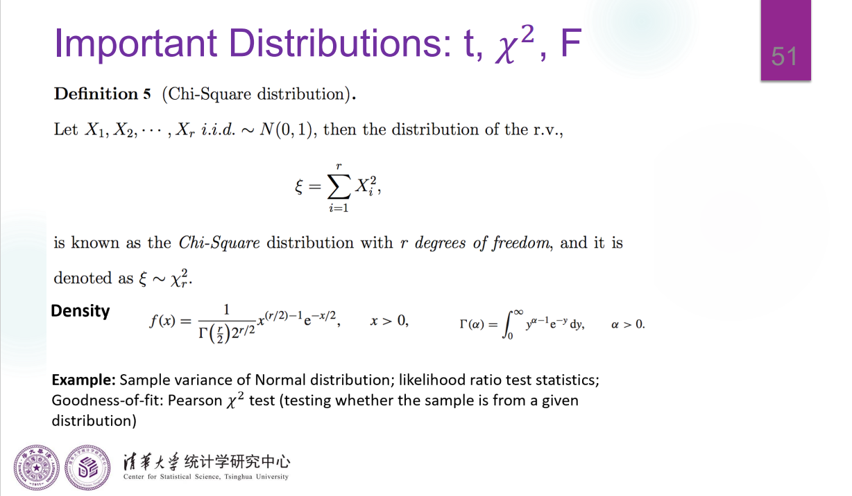
经典分布查阅

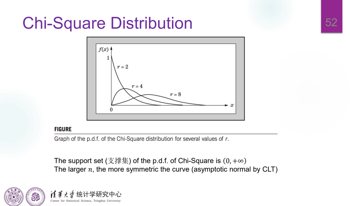
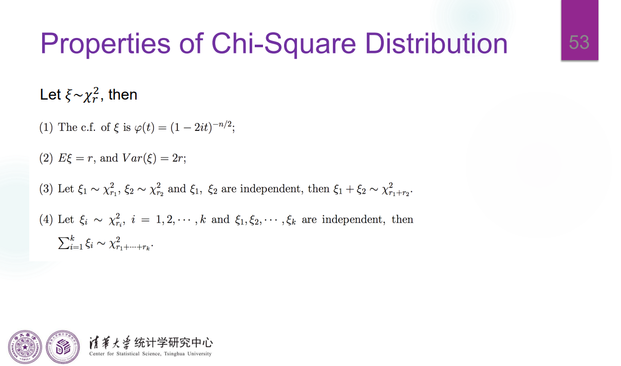
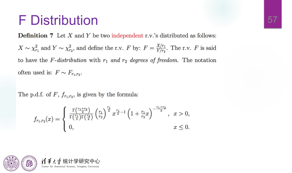
卡方分布

\(t-\)分布

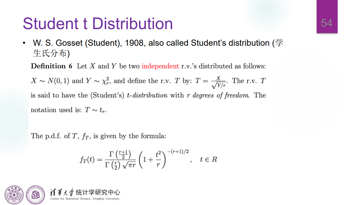
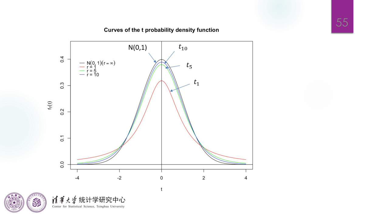
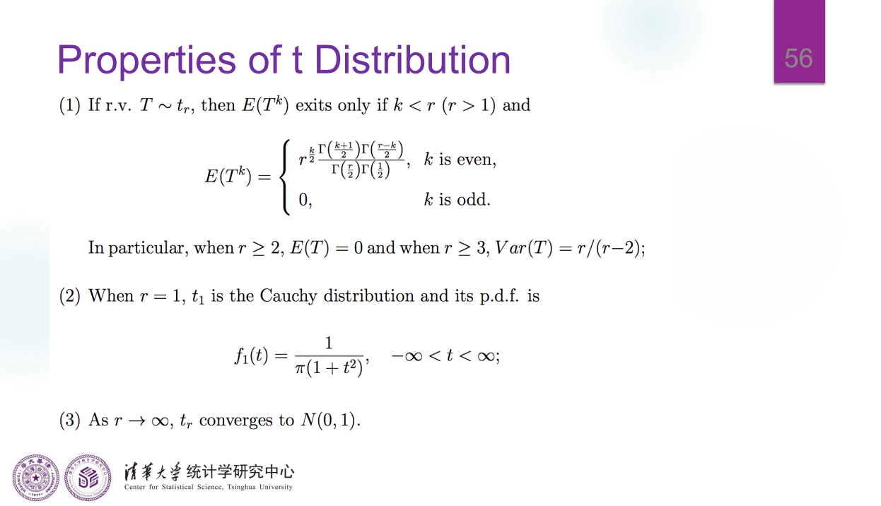
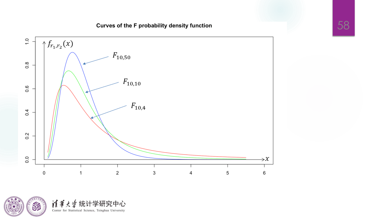
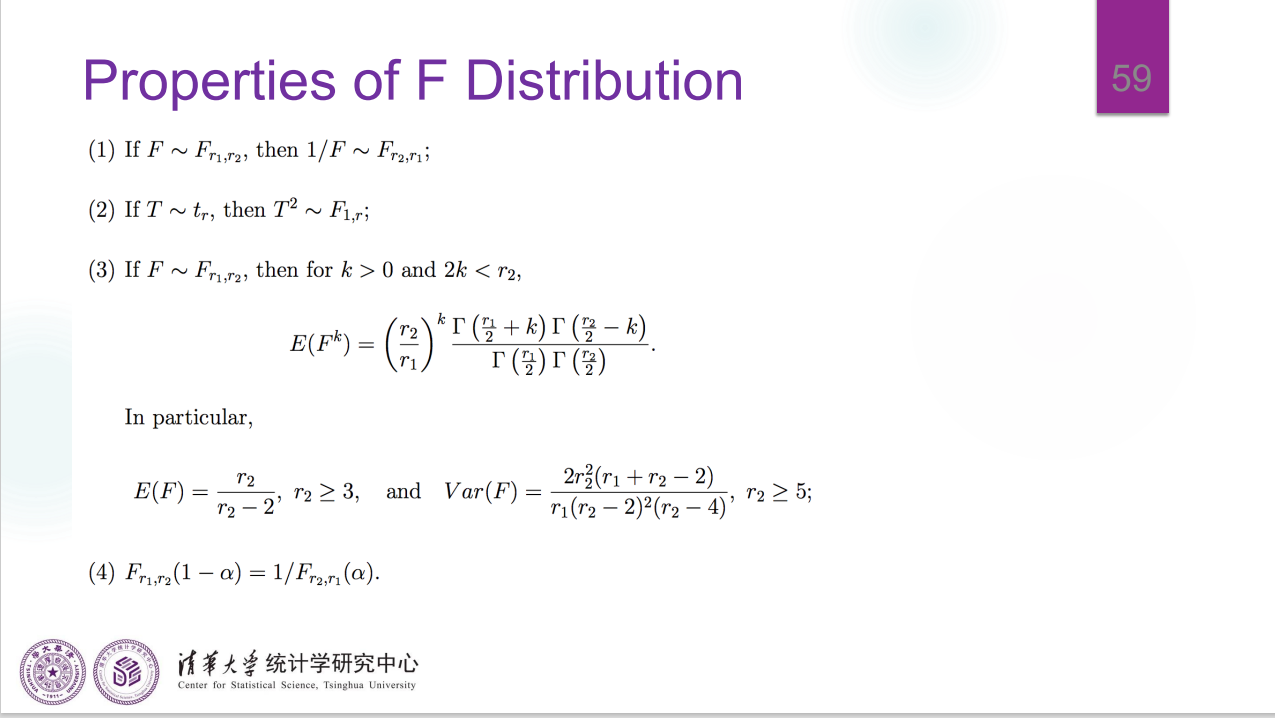
\(F\) 分布

Lecture 2

本节仍然是介绍统计学的基础内容，讨论了一些 Statistic 的性质，并介绍了分布族。

我偷懒，定理和证明就直接拍手写了，自认为自己的字还没那么不堪入目。另外每个学期都会有找不到的笔记，还是存电子版吧（

统计量及其性质

Lecture 1 中介绍了 114514 个常用的 Statistic，我们对其中一些讨论它们的 sample distribution 的性质。

特殊统计量

• Sample mean：因为它的形式是 \(nX = X_1+X_2+...+X_n\)，且 \(X_i\) 互相之间 i.i.d.，我们可以用概率母函数 / 矩母函数来处理得到 \(nX\) 的分布。

  如果只是求近似而不是准确的分布，可以使用 Central Limit Theorem 进行估计，但要注意，只有 \(X_i\) 的方差有限的情况才能使用 CLT。

• Linear transformation：形为 \(Y=\frac{X}{n}\)，于是我们可以用 \(CDF\) 转 \(PDF/PMF\) 的方式计算它的 \(PDF/PMF\)，直接给出结论：\(f_Y(y)=nf_X(ny)\)。

经典结论

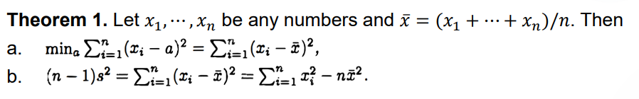
• Theorem 1：

  

• Theorem 2：

  

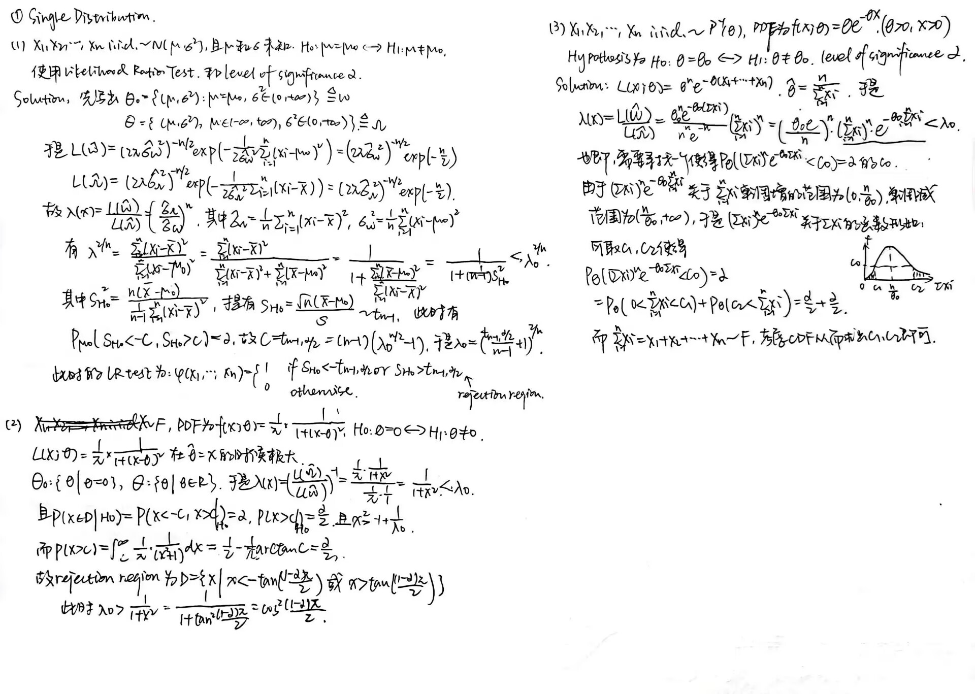
  这个第二问的证明，要用一下 \(cov(X_1,X_2)=0\)，权当留个提示。因为我第一遍没证出来。

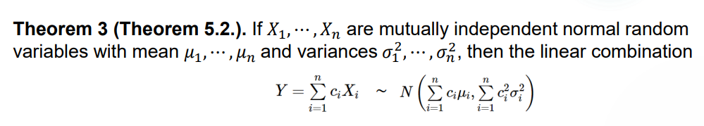
• Theorem 3：

  

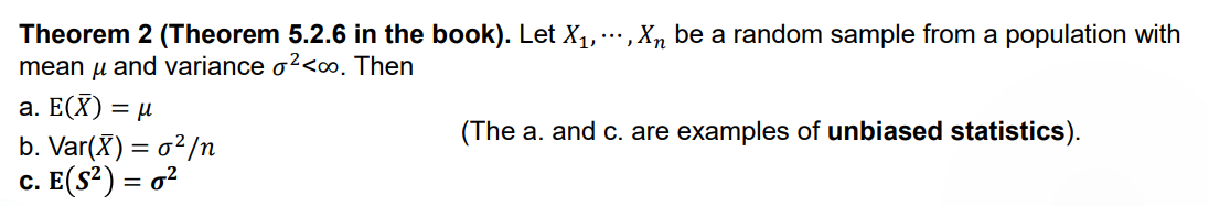
  因为 \(\bar{X}\) 的期望和 \(X_1\) 的期望相同，\(S\) 的期望和 \(X_1\) 的方差相同，因此二者是 unbiased statistic（无偏统计量）

正态分布的随机抽样

• Theorem 1：考虑独立不同分布的正态分布的线性组合，它的方差和期望也是一个线性组合。一般这种类似于 \(X_1+X_2+...+X_n\) 的都可以用矩母函数证明。

  

• Example 1：

  

  \(X,Y\) 是两个方差和期望都已知的正态分布，要求 \(P(X>Y)=P(X-Y>0)\)，而 \(X-Y\) 是正态分布的线性组合，也是参数已知的正态分布，将其标准化即可。

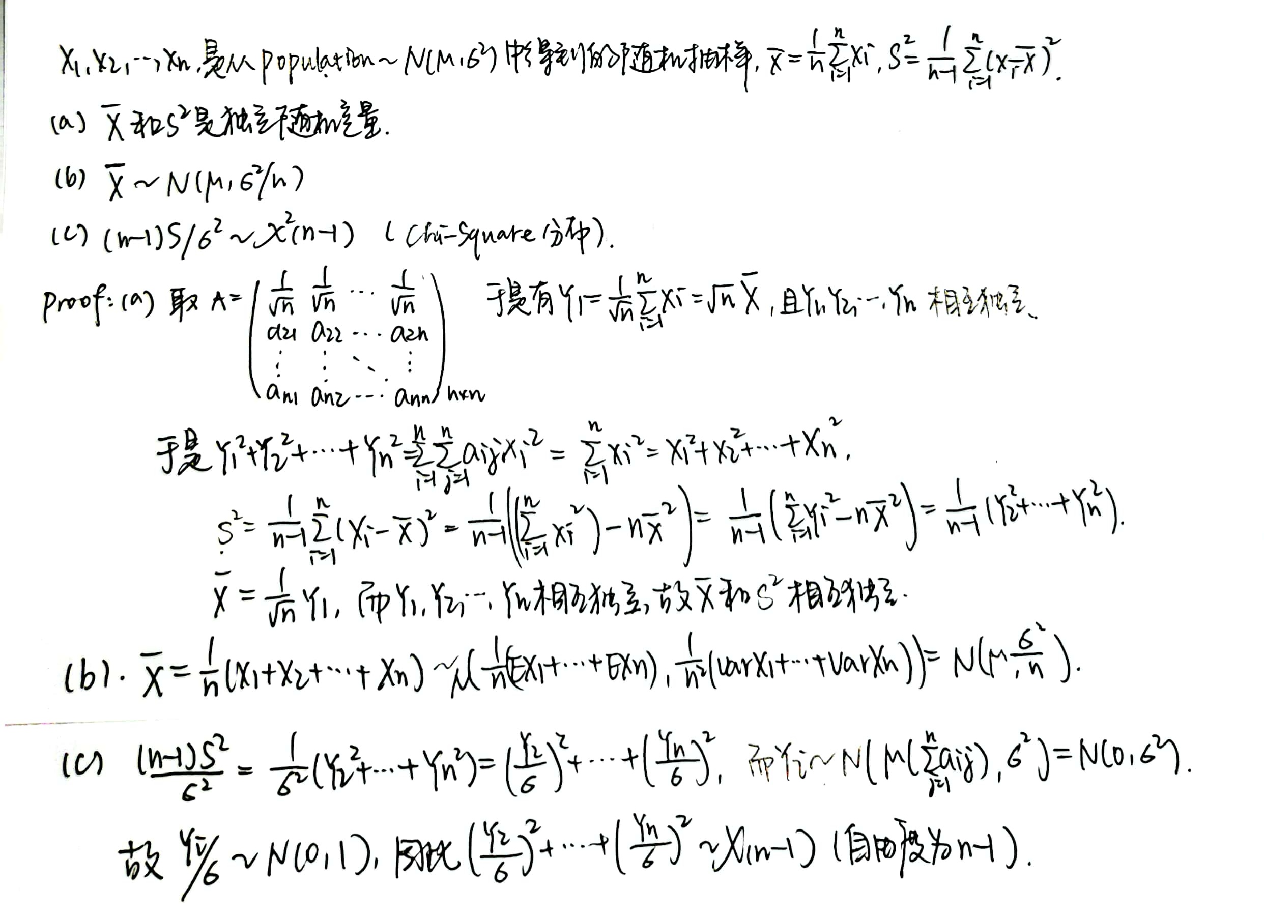
• Theorem 2：考虑一组由正态分布随机抽样生成的 statistics，用矩阵形式表示：

  

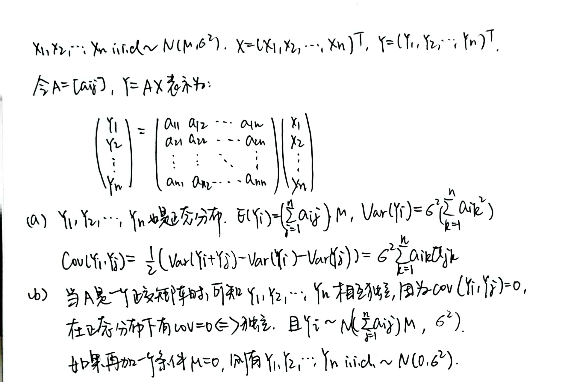
  可以看到矩阵是正交矩阵时有很好的性质。固定正交矩阵的第一行之后，我们可以对此时的 \(\bar{X}\) 和 \(S^2\) 进行讨论：

  Theorem 3：\(\bar{X}\) 和 \(S^2\) 是独立的，且由 \(S^2\) 可以生成一个 Chi-Square 分布。

  

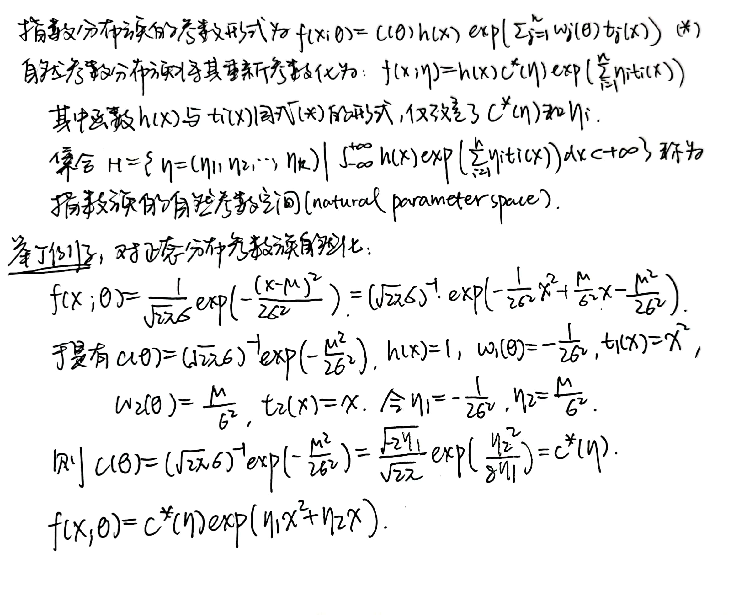
指数分布族

概念

• 简单来说，一个分布的 PDF / PMF 可以表示为 \(f(x; \theta) = c(\theta)h(x) exp[\Sigma_{j=1} ^{n} w_j(\theta) t_j(x)]\) 的形式，则无论随机取多少个独立同分布的 sample，它们的联合分布也可以保持这个形式，则称该 population 属于指数分布族。

  其中的 \(\theta\) 表示该分布的参数，可以表示为 \(\theta = (\theta_1,\theta_2,...,\theta_k)\)

  比如正态分布，Poisson 分布都属于指数分布族：

  \(f(x_1,x_2,...,x_n;\theta) = (\sqrt{2\pi} \sigma)^{-n} exp(-\frac{1}{2\sigma ^2} \Sigma_{i=1} ^{n} (x_i-\mu)^2)\) 为正态分布的 Joint PDF；

  \(f(x_1,x_2,...,x_n;\theta) = e^{-n\theta} (\Pi_{i=1} ^{n} \frac{1}{x_i !}) exp(ln\theta (x_1 + x_2 +...+ x_n))\) 为泊松分布的 Joint PMF。

  实际上，连续的指数分布族还有 Gamma，Beta 分布族，离散的指数分布族还有二项和负二项分布族。

自然指数分布族

• 自然指数分布族和举例：

  

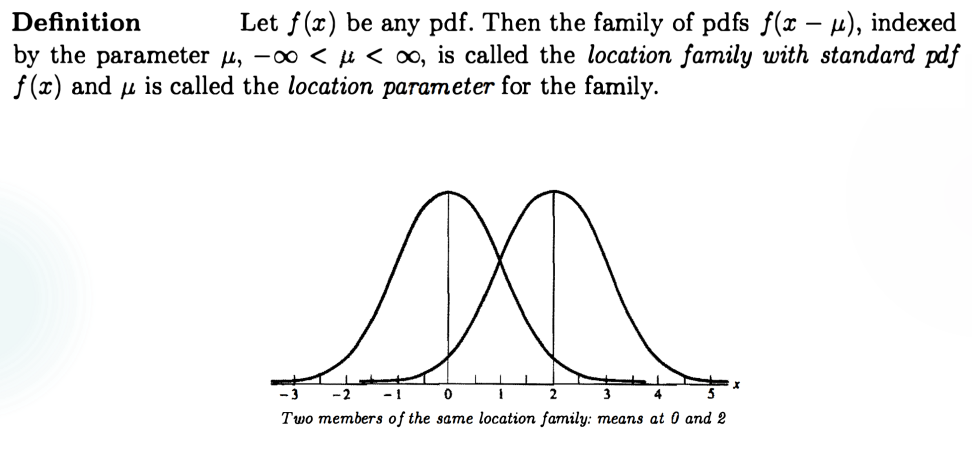
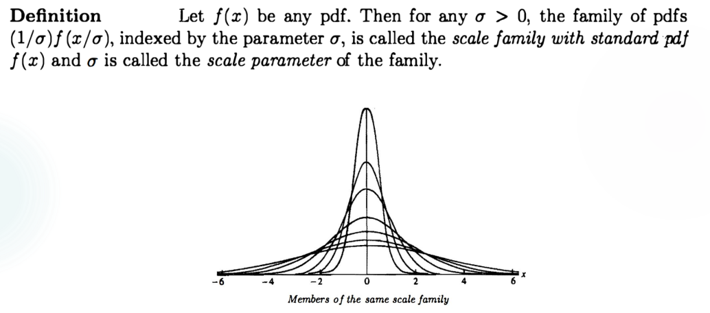
位置与尺度族

• 位置与尺度族：直观来说，位置族的形状完全一样，但位置上有偏移，例如若干个期望不同而方差相同的正态分布；尺度族的位置相同，形状上有伸缩变化，例如若干个期望相同但方差不同的正态分布。

• 位置族：取一个标准概率密度函数（standard PDF）\(f(x)\)，位置族中的其他函数 \(f(x-\mu)\) 相对于这个标准函数的偏差记为 \(\mu\)，称为 location parameter（位置参数）.

  

• 尺度族：取一个标准概率密度函数（standard PDF）\(f(x)\)，尺度族中的其他函数 \(\frac{1}{\sigma} f(\frac{x}{\sigma})\) 相对于这个标准函数的偏差记为 \(\sigma\)，称为 scale parameter（尺度参数）.

  

• 位置-尺度族：取一个标准概率密度函数（standard PDF）\(f(x)\)，位置-尺度族中的其他随机变量 \(X\) 有 PDF 为 \(\frac{1}{\sigma} f(\frac{x-\mu}{\sigma})\) ，当且仅当存在以 \(f(z)\) 为 PDF 的随机变量 \(Z\)，从而有 \(X=\sigma Z+\mu\)。

  这一定理可以用 CDF 法证明。

• 例子：\(Z\sim N(\mu,\sigma ^2)\)，且 $X=aZ+b $，于是 \(X\sim N(a\mu +b,a^2 \sigma ^2 )\)，相对于 standard distribution \(Y\sim N(0,1)\)，location parameter 为 \(a\mu +b\)，scale parameter 为 \(a\sigma\)。

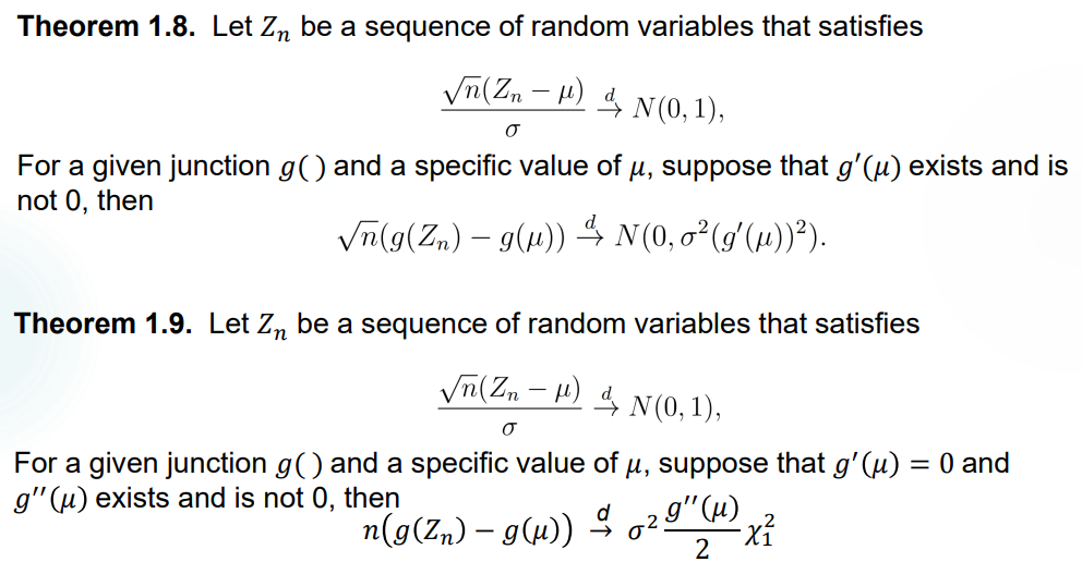
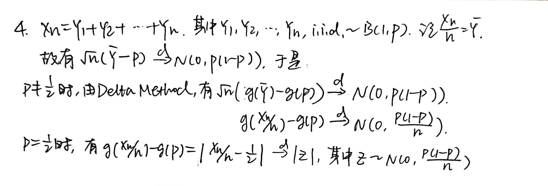
Delta Method (Application Only)

就两个定理，也没证明。用于已知参数的分布 \(X\) 的函数 \(g(X)\)，对其进行近似。第一个定理针对 \(g'(\mu) \neq 0\)，第二个定理针对 \(g'(\mu)=0\) 的情况进行进一步近似。

其他定理查阅

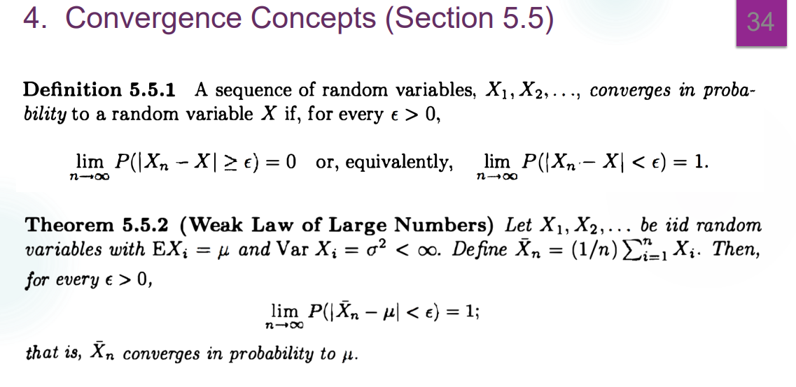
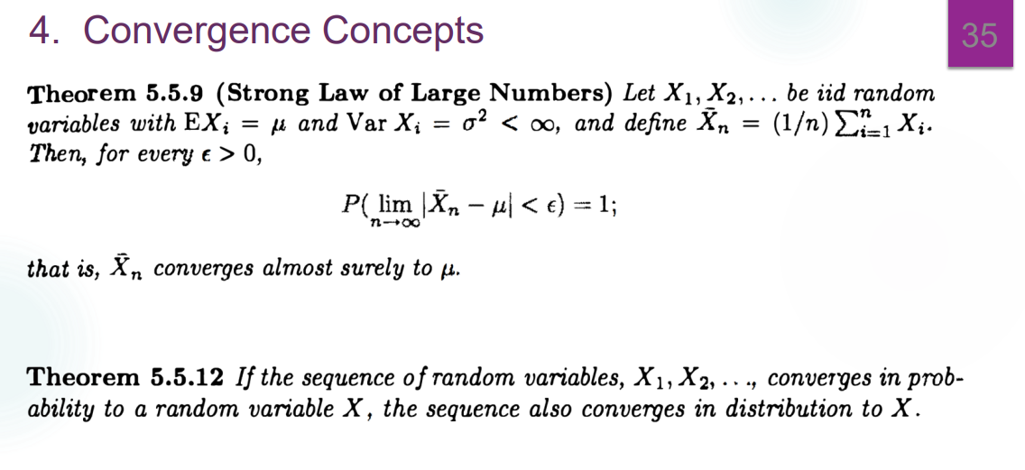
大数定律

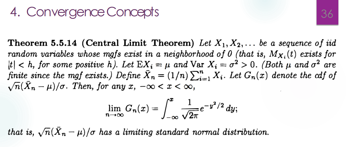
中心极限定理

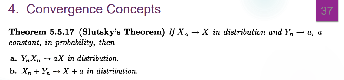
Slutsky's Theorem

Homework 1

Lecture 3

本节介绍数据简化原理，仍然围绕 Statistic 的选取展开。

Data don't make any sense, we will have to resort to statistics.

然而，每一个 statistic 的使用都不可避免地会遗失数据的细节。这些细节有时是没有用的，statistic 反而保留了最有用的部分（例如 parameter）；有的时候是有用的，根据数据处理的目的，有可能需要重新选择 statistic。

充分统计量

定义和应用

• Sufficient statistics：\(T(x)\) 是一个充分统计量当且仅当样本 \(X\) 在 \(T(X)\) 条件下的分布与 \(\theta\) 无关。

  写作数学语言：\(P_\theta(X=x | T(X)=T(x)) = \frac{P_\theta (X=x)}{P_\theta(T(X)=T(x))} = \frac{p(x;\theta)}{q(T(x);\theta)}\) 与参数 \(\theta\) 无关。于是，验证一个 statistic \(T(x)\) 最直接的方法就是计算 \(x\) 的联合分布的概率密度，以及 \(T(x)\) 的概率密度，对二者求比值。

• 对一些特殊的分布，我们来寻找它们的充分统计量。

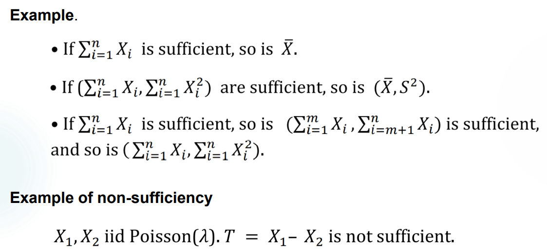
  • Bernoulli sufficient statistic：\(X_1,X_2,...,X_n i.i.d\sim B(1,\theta)\)，则 \(T(X)=X_1+...+X_n\) 是 \(\theta\) 的充分统计量，可以通过 \(T(X)\sim B(n,\theta)\) 来验算。

  • Normal sufficient statistic：\(X_1,X_2,...,X_n i.i.d\sim N(\mu,\sigma^2)\)，则 \(T(X)=\bar{X}\) 是 \(\mu\) 的充分统计量（注意不是 \(\sigma\) 的充分统计量），可以通过 \(T(X)\sim N(\mu,\frac{\sigma^2}{n})\) 验算。

  • Sufficient order statistic：\(X_1,X_2,...,X_n i.i.d\)，population 的 PDF 是 \(f(x)\)，于是全体次序统计量 \(X_{(1)},...,X_{(n)}\) 是充分统计量，因为 \(P(X_1=x_1,...,X_n=x_n | X_{(1)}=x_{(1)},...,X_{(n)}=x_{(n)}) = \frac{1}{n!}\)

    Remark：这提示我们，次序统计量可以是多维的。

• 显然，这样寻找充分统计量是不现实的。以下有因子分解定理帮助我们寻找合适的 \(T(x)\)：

  Factorization theorem：设 $f(x;) $ 是 sample X 的联合概率密度函数，统计量 \(T(x)\) 是 sufficient statistic 当且仅当存在函数 \(g(t;\theta)\) 和 \(h(x)\)，满足 \(f(x;\theta)=g(T(x);\theta)h(x)\)。

  对离散条件的 Factorization theorem 进行证明：

  左推右，trivial。右推左：

  

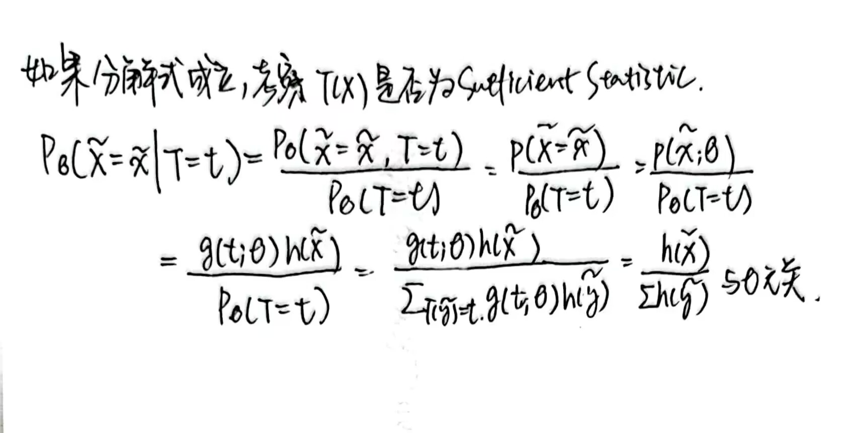
• 因此，由 Factorization theorem 可以知道，把 Joint PDF 里面 \(\theta,\bar{x}\) 不可分离的部分，以及 \(\theta\) 单独的部分取出放在一起，就可以从中找出 sufficient statistic。

• 应用数理统计的概率写法，求充分统计量

  • Uniform sufficient statistic：\(X_1,X_2,...,X_n i.i.d\sim Unif(\theta_1,\theta_2)\)，寻找关于 \(\theta_1,\theta_2\) 的充分统计量。

    事实上，Joint PDF 可以写成 \(f(x_1,x_2,...,x_n)=(\frac{1}{\theta_2-\theta_1})^nI_{\lbrace\theta_1 \leq x_1,x_2,...,x_n \leq \theta_2\rbrace}\)，也即

    \(f(x_1,x_2,...,x_n)=(\frac{1}{\theta_2-\theta_1})^nI_{\theta_1 \leq x_{(1)}}I_{x_{(n)} \leq \theta_2}\)，于是 sufficient statistic 是 \(x_{(1)},x_{(2)}\)。

  • Exponential sufficient statistic：\(X_1,X_2,...,X_n i.i.d\sim exp(\lambda)\)，寻找关于 \(\lambda\) 的充分统计量。

    事实上，Joint PDF 是 \(f(\bar{x};\lambda)=\lambda^n e^{-\lambda(x_1+...+x_n)}=\lambda^ne^{-\lambda t} h(\bar{x})=g(t;\lambda)h(\bar{x})\)，于是有 \(T(\bar{X})=X_1+X_2+...+X_n\) 是 sufficient statistic，而 \(h(\bar{x})=I_{x_i>0,i=1,2,...,n}\)。

  • 还有很多例子，懒得举了

• Exponential family 的 PDF 有比较好的性质： \(f(x; \theta) = c(\theta)h(x) exp[\Sigma_{j=1} ^{n} w_j(\theta) t_j(x)]\)

  于是 Joint PDF 可以写为 \(f(\bar{x}; \theta) = c(\theta)^m \Pi_{i=1}^m h(x_i) exp[\Sigma_{j=1} ^{n} \Sigma_{i=1} ^m w_j(\theta) t_j(x_i)]\)，因此这一样本的充分统计量是 \((\Sigma_{j=1}^m t_1(X_j),...,\Sigma_{j=1}^m t_n(X_j))\)。

充分统计量的性质

• \(T\) 是参数 \(\theta\) 的充分统计量，且 \(T=\phi(S)\)，则 \(S\) 也是充分统计量。
  • 如果 \(\phi\) 是一一对应，二者的信息量相同。
  • 如果 \(\phi\) 不是一一对应，则 \(T\) 是 \(S\) 的一个精简而且还是充分统计量，是更有用的。
  
• Examples（懒得抄了）：

极小充分统计量

• sufficient statistic \(T^*(X)\) 被称为 minimal sufficient statistic 当且仅当：对任意充分统计量 \(T(X)\)，存在函数 \(\psi\) 使得 \(T^*(X)=\psi(T(X))\)。也就是说，\(T^*(X)\) 实现了数据的最大简化。minimal sufficient statistic 的维度是最小的，它不一定唯一。

  • 判定定理：\(f(x;\theta)\) 是 \(X\) 的 PDF，则对两个样本点 \(x\) 和 \(y\)，\(f(x;\theta)/f(y;\theta)\) 是 \(\theta\) 的常函数当且仅当 \(T(x)=T(y)\)，那么 \(T(X)\) 是 \(\theta\) 的 minimal sufficient statistic。证明如下：

  

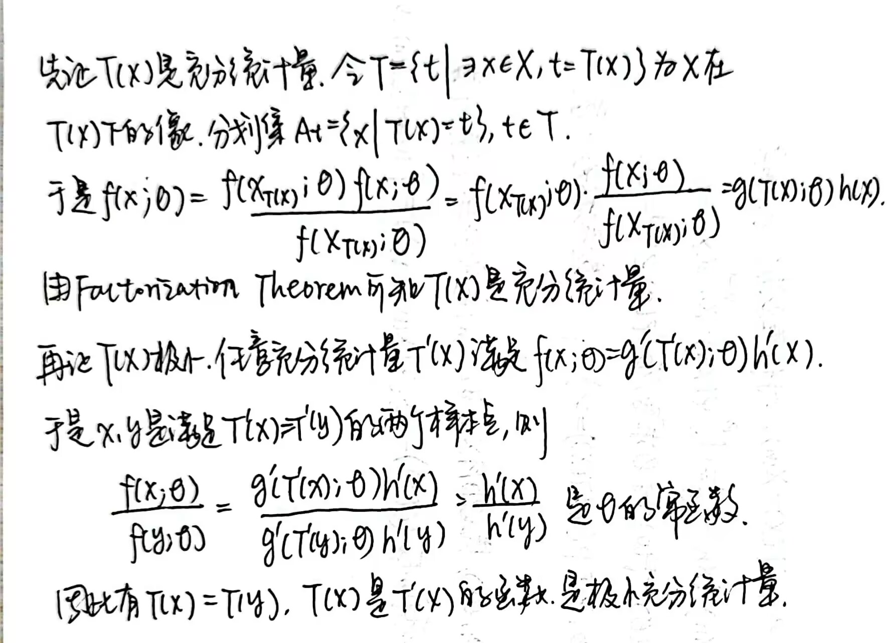
• 举一些例子。

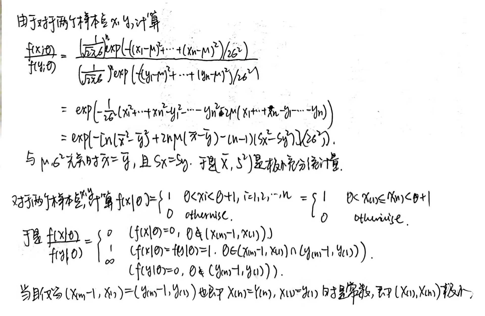
  • Normal minimal sufficient statistic：\(X_1,X_2,...,X_n i.i.d\sim N(\mu,\sigma^2)\)，则 \((\bar{X},S^2)\) 是 \((\mu,\sigma^2)\) 的极小充分统计量。

  • Uniform minimal sufficient statistic：\(X_1,X_2,...,X_n i.i.d\sim Unif(\theta,\theta +1)\)，则 \((X_{(1)},X_{(2)})\) 是 $$ 的极小充分统计量。

  • 分别验证如下：

    

辅助统计量

定义

• \(S(X)\) 是 ancillary statistic 当且仅当它的分布是 \(\theta\) 的常函数。比如说，常数就是一个 trivial ancillary statistic。

• \(S(X)\) 是一阶 ancillary statistic，当 \(E(S(X))\) 也是 \(\theta\) 的常函数时。

• 举一些例子：

  • Uniform ancillary statistic：\(X_1,X_2,...,X_n i.i.d\sim Unif(\theta,\theta+1)\)，则 \(X_{(n)}-X_{(1)}\) 是辅助统计量。验证如下：

  • Location ancillary statistic：\(Z_1,Z_2,...,Z_n\) 是服从 \(F(x)\) 的 Population 中的样本，位置参数为 \(\theta\)，于是 \(X_1=Z_1+\theta,...,X_n=Z_n+\theta\)，故 \(r=X_{(n)}-X_{(1)}\) 是 ancillary statistic，因为

    $F(r;)=P(Rr;)=P(maxX_i-minX_i r)=P(max Z_i-minZ_i r)=P(Z_{(n)}-Z_{(1)}r) $

    这是和 \(\theta\) 无关的量。所以，location ancillary statistic 还可以是 \(X_{(n-1)}-X_{(3)}\)，等等。

  • Scale ancillary statistic：同理，\(X_i/X_j\) 都是 ancillary statistic，因为可以归一为 \(Z_i/Z_j\)。由统计量的函数性质可知，\(\frac{X_1+...+X_n}{X_i}\) 是形式比较好的 ancillary statistic。

辅助统计量的性质

• \(V(X)\) 是 nontrivial ancillary statistic，于是 \(\lbrace x:V(x)=v\rbrace\) 不包含任何 \(\theta\) 的信息。
• \(T(X)\) 是 statistic，如果 \(V(T(X))\) 是 nontrivial ancillary statistic，那么 \(T\) 的简化中仍然不含有 \(\theta\)，需要进一步进行简化。
• 如果一个 sufficient statistic \(T(X)\) 没有非常值函数是 ancillary statistic，那么它在简化数据中是最优的。

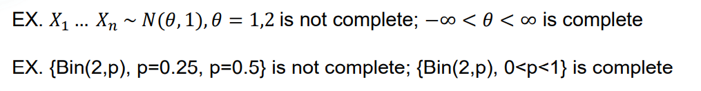
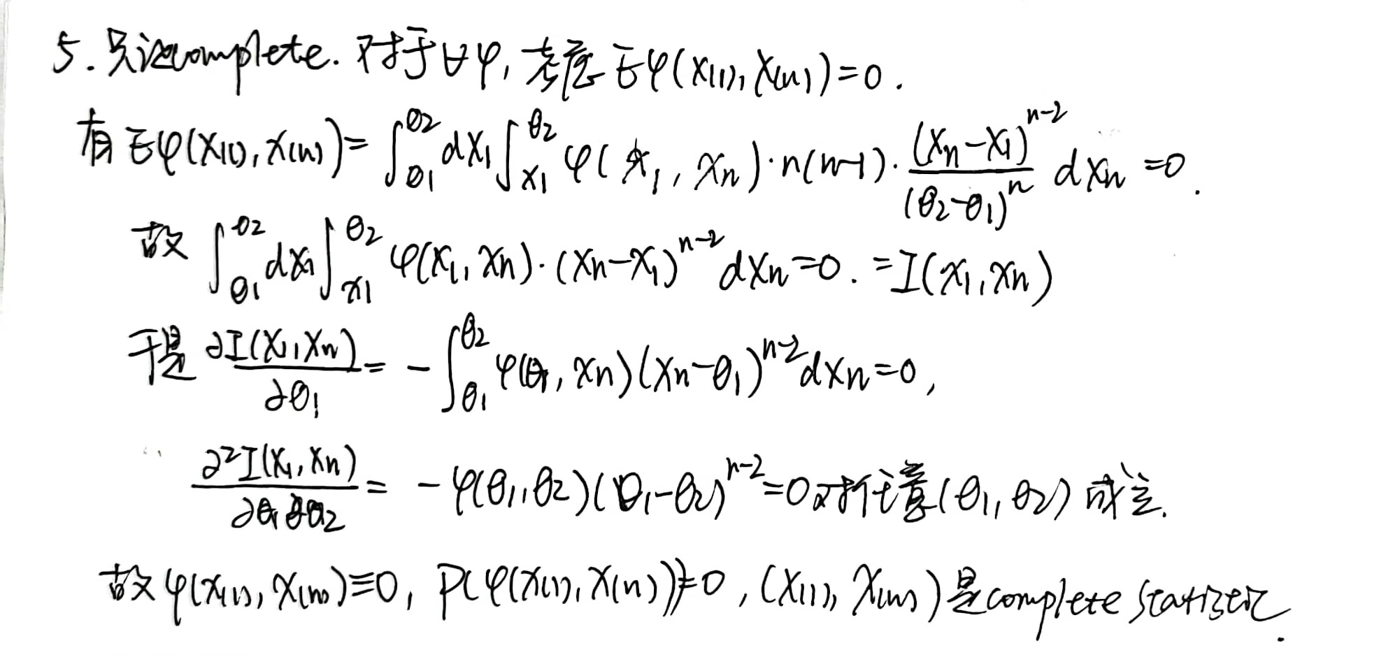
完全统计量

定义

• \(X\sim F=\lbrace f(x;\theta),\theta \in \Theta \rbrace\) 是一个分布族，\(\Theta\) 是参数空间。记 \(T=T(X)\)，如果对于任意函数 \(\psi\)，如果 \(E_\theta \psi(T(X))=0,\forall \theta \in \Theta\)，那么一定有 \(P_\theta(\psi(T(X))=0)=1,\forall \theta \in \Theta\)。

• 听起来很抽象，举几个例子：

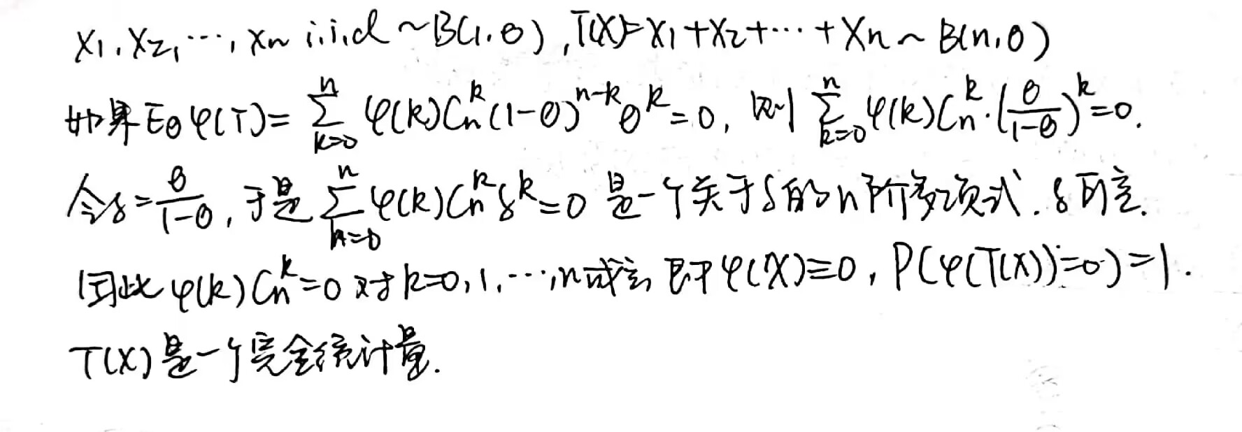
  • \(X=(X_1,X_2,...,X_n)\) 是来自于 \(B(1,\theta)\) 的随机样本，那么 \(T(X)=\Sigma_{i=1} ^n X_i\) 对于参数 \(\theta\) 是一个 complete statistic。验证如下：

    

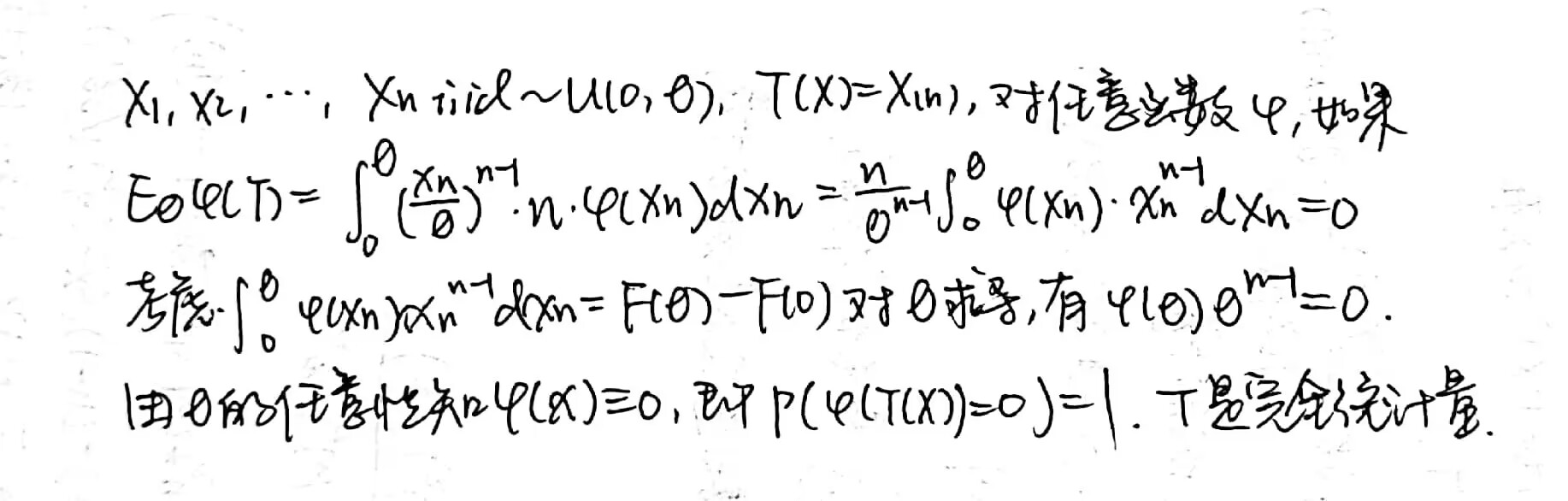
  • \(X=(X_1,X_2,...,X_n)\) 是来自于 \(Unif(0,\theta)\) 的随机样本，那么 \(T(X)=X_{(n)}\) 对于参数 \(\theta\) 是一个 complete statistic。验证如下：

    

• complete statistic 不一定存在。

指数族中的完全统计量

• 指数分布族的 PDF 有形式： \(f(x; \theta) = c(\theta)h(x) exp[\Sigma_{j=1} ^{n} w_j(\theta) t_j(x)]\)

  于是如果参数空间 \(\Theta\) 包括 \(R^k\) 的开集，则统计量 \(T(X)=(\Sigma_{i=1} ^m t_1(X_i),...,\Sigma_{i=1} ^m t_n(X_i))\) 是一个 complete statistic。

• Remark：定理中要求开集是为了防止一些特殊情况，比如：

完全统计量的性质

• 如果 minimal sufficient statistic 存在，那么任何 complete statistic 都是 minimal sufficient 的。

• Basu Theorem：如果 \(T(X)\) 是 (minimal) complete & sufficient statistic，那么它和任何 ancillary statistic 独立。这是一个很好的性质，因为直观上来看 ancillary statistic 是和任何 sufficient statistic 独立的而现实并非如此，而这个定理可以给出一个补充条件。

• Basu Theorem 的应用：

  • 设 \(X_1,...,X_n i.i.d\sim U(\theta_1,\theta_2)\)，证明 \(\frac{X_{(i)} - X_{(1)}}{X_{(n)}-X_{(1)}}\) 与 \((X_{(n)},X_{(1)})\) 独立。

    \(X_{(n)}\) 是 complete statistic，\((X_{(n)},X_{(1)})\) 是 minimal sufficient statistic，于是也是 minimal complete & sufficient statistic，只要证明 \(\frac{X_{(i)} - X_{(1)}}{X_{(n)}-X_{(1)}}\) 是 ancillary statistic 即可。

    而这是一个位置-尺度分布族，需要先正规化为 \(Y_i = \frac{X_i-\theta_1}{\theta_2-\theta_1}\)，则有 \(Y_1,Y_2,...,Y_n i.i.d.\sim U(0,1)\)，于是 \(\frac{X_{(i)} - X_{(1)}}{X_{(n)}-X_{(1)}}=\frac{Y_{(i)}-Y_{(1)}}{Y_{(n)}-Y_{(1)}}\)，从而是 \(\theta\) 的常函数，为 ancillary statistic。

  • 设 \(X_1,...,X_n i.i.d\sim N(\mu,\sigma^2)\)，证明 \(\bar{X}\) 和 \(S^2\) 是独立的。

    实际上，这个问题在 Lecture 2 中我们使用正交矩阵证明过，此处再给出一个 Basu Theorem 下的证明。事实上，我们已经知道对于已知的 \(\sigma^2\)，有 \(\bar{X}\) 是 complete & sufficient，而 \(S^2\) 是 ancillary，所以二者独立。

似然原理

• 如果 \(f(x;\theta)\) 是样本 \(X=(X_1,X_2,...,X_n)\) 的 Joint PDF，则记 \(\theta\) 的函数 \(L(\theta;x)=f(x;\theta)\) 为似然函数（Likelihood Function），有时也写作 \(L(\theta)\) 以突出变量。

  Log Likelihood：\(l(\theta;x)=log L(\theta;x)\)。

• Likelihood Principle：

  • 用参数族 \(\Theta\) 中的不同参数 \(\theta_1,\theta_2\) 进行比较 \(L(\theta_1;x)>L(\theta_2;x)\)，那么 \(\theta_1\) 比起 \(\theta_2\) 是一个更好的真实值的选择。从而可以在参数未知的情况下，对真实的 \(\theta\) 进行推断。
  • 样本点 \(x,y\) 满足 \(L(\theta;x)\) 和 \(L(\theta;y)\) 之间成比例，即存在 \(L(\theta;x)=C(x,y)L(\theta;y)\)，那么从 \(x,y\) 出发对 \(\theta\) 做如上推断，得到的结果是相同的。

• Equivalence Principe：如果 \(Y=g(X)\) 是一个度量尺度变换，且 \(Y\) 的模型和 \(X\) 的模型具有相同的形式结构，则推断方法应同时满足度量同变和形式不变。

Lecture 4

本节介绍 Fisher Information 和 Point Estimation。

Fisher Information

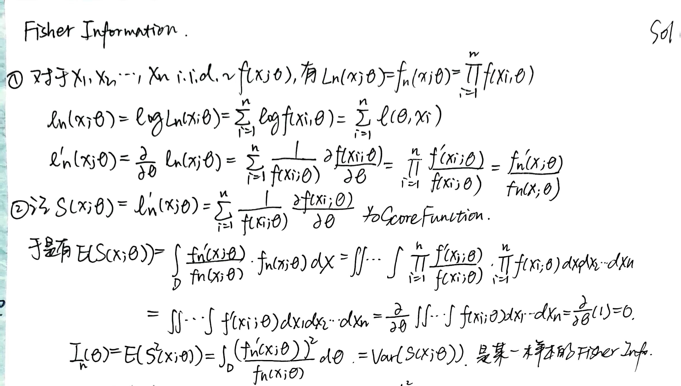
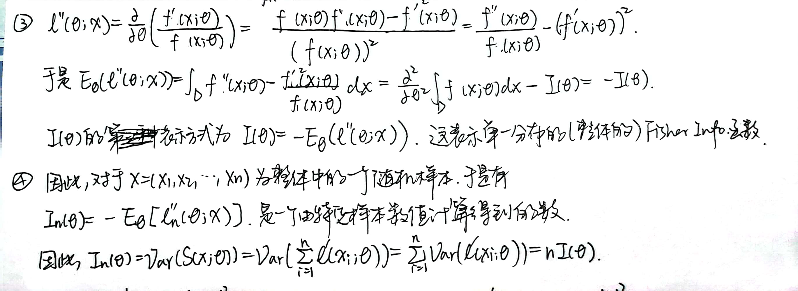
定义

• 取 \(f(x;\theta),\theta \in \Theta\) 作为一个分布族，则 score function 定义为 \(S(x;\theta)=\frac{\partial log L(\theta)}{\partial \theta}=\frac{1}{f(x;\theta)} \frac{\partial f(x;\theta)}{\partial \theta}\)。

  对于一个给定的 \(\theta\)，可知 \(E[S(X,\theta)]=0,E[S(X,\theta)]^2=I(\theta)\)，后者就是 Fisher Information。

  因此，\(Var[S(X;\theta)]=E[S(X;\theta)]^2- E^2[S((X;\theta))]=I(\theta)\)

  对于一个 score function 有较大方差的分布，我们希望能够较为容易地估计 \(\theta\)。

• \(I(\theta) = E[S(X;\theta)]^2 = -E(\frac{\partial^2}{\partial \theta^2} logL(\theta))\)

与熵的关系

• relative entropy：\(KL(p:q)=\int p(x)log \frac{p(x)}{q(x)} dx\)，

  定义：

  \(D(\theta,\theta + \Delta \theta)=KL(f(x;\theta):f(x,\theta+\Delta \theta)) = -\int f(x;\theta)[log f(x,\theta + \Delta \theta)-log f(x;\theta)] dx\)

  经过 Taylor 展开：

  \(log f(x,\theta + \Delta \theta)-log f(x,\theta) = \frac{\partial log f(x,\theta)}{\partial \theta} \Delta \theta + \frac{1}{2} \Delta \theta^\prime \frac{\partial^2 log f(x,\theta)}{\partial \theta^\prime \partial \theta} \Delta \theta + o(||\Delta \theta||^2)\)

  于是：

  \(D(\theta,\theta+\Delta \theta) = -E[\frac{\partial log f(x,\theta)}{\partial \theta}]\Delta \theta - \frac{1}{2} \Delta \theta^\prime E[\frac{\partial^2 log f(x,\theta)}{\partial \theta^\prime \partial \theta} ]\Delta \theta + o(||\Delta \theta||^2) = -\frac{1}{2}\Delta \theta^\prime I(\theta) \Delta \theta\)

  Remark： Fisher Information 越大，越能够区分参数。

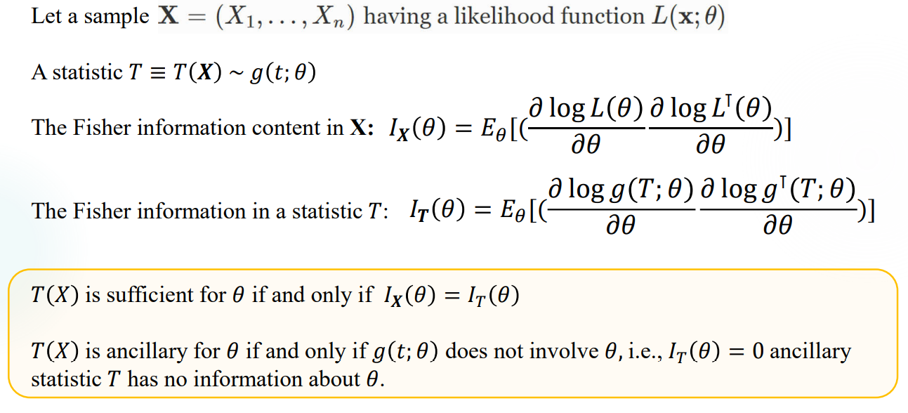
充分统计量和辅助统计量

不是很懂。贴个图吧。

点估计

定义

• Example 1：\((X_1,X_2,...,X_n)i.i.d \sim N(\mu,\sigma^2)\)，我们想找到两个参数比较好的一个估计，可以考虑 \(\mu = \bar{X},\sigma^2 = S^2\)。这是非常典型的估计量，因为 \(E(\bar{X})=\mu,E(S^2) =\sigma^2\) ，因此是无偏的。
• Example 2：\((X_1,X_2,...,X_n)i.i.d \sim P(\lambda)\)，于是考虑 \(P(X_1=x_1,...,X_n=x_n)\)可知 \(T(X)= X_1+...+X_n \sim P(n \lambda )\) 是一个充分统计量，\(E(T(X))=\lambda\)。
• 实际上，样本的任意一个 statistic 都是它的点估计量（point estimator），实际观测值称为估计值，即 estimate，它是一个数值。

好的性质

• 无偏性。对于 population \(\lbrace f(x;\theta):\theta \in \Theta \rbrace\) 中的随机抽样 \(X=(X_1,...,X_n)\)，\(g(\theta)\) 是定义在参数空间 \(\Theta\) 上的函数，一个 \(g(\theta)\) 的估计量，\(\hat{g}(X)=\hat{g}(X_1,...,X_n)\) 是 unbiased 如果 \(E_\theta [\hat{g}(X)]=g(\theta),\theta \in \Theta\)。否则是有偏的。

  定义 systematic error 为 \(E(\theta)-\theta\)，则无偏即为 systematic error 为 0.

  说句人话，就是求某个 estimator 的期望是不是 \(\theta\)，如果是的话就是无偏的。

• 有效性。对于两个 estimators \(\hat{g}_1(X),\hat{g}_2(X)\)，如果 \(Var(\hat{g}_1(X))\leq Var(\hat{g}_2(X))\) 对任意 \(\theta \in \Theta\) 成立，并且参数空间中至少有一个 \(\theta\) 使上述式子不取等号，那么称 \(\hat{g}_1 (X)\) 相比 \(\hat{g}_2(X)\) 更有效。

• 相合性。

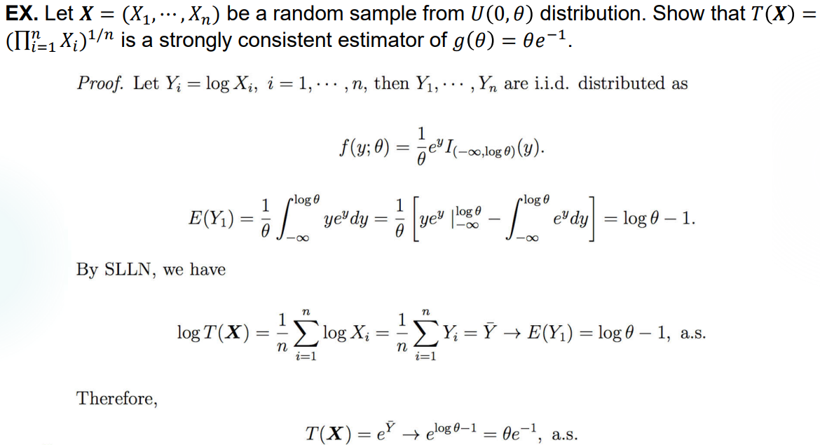
  • 对任意样本量为 \(n\) 的样本，记 \(\hat{g}_n(X) = \hat{g}_n (X_1,...,X_n)\) 是一个 estimator，如果 \(\hat{g}_n(X)\) 依概率收敛到 \(g(\theta)\)，也即，对任意的 \(\theta \in \Theta\)，\(\varepsilon >0\)，有 \(\lim_{n\to \infty} P_\theta (|\hat{g}_n (X) -g(\theta)| \geq \varepsilon)=0\)，那么 \(\hat{g}_n(X)\) 被称为一个 \(g(\theta)\) 的 weakly consistent estimator。

  • 如果对任意 $$，有 \(P_\theta (lim _{n \to \infty} \hat{g}_n (X)=g(\theta))=1\)，则称其为 strongly consistent estimator。

  • 如果对任意 \(\theta \in \Theta ,r>0\)，有 $lim {n } E|_n(X)-g()|^r = 0 $，则称其为 \(g(\theta)\) 的 \(r\) 阶 consistent estimator。

  • Example 1：（这个对我来说还是一下子难以想到..归根结底是初概这一部分没学会，要补）

    

评价点估计的方式——MSE

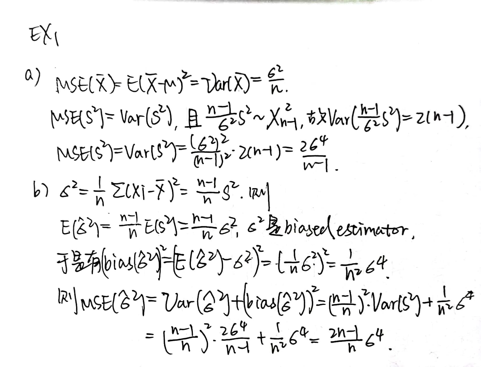
• Mean Squared Error（MSE）：对于一个 estimator \(T\) 和一个参数 \(\theta\)，MSE 定义为：

  \(MSE(T)=MSE_\theta(T)=E_\theta((T-\theta)^2)=Var_\theta(T)+(Bias_\theta (T))^2\)，

  其中，\(Bias_\theta (T)=E_\theta(T)-\theta\)。于是对于一个无偏的 \(T\)，它的 MSE 就是方差。

• 如果有某个 \(\hat{g}^*(X)\) 使得对任意的 estimator \(\hat{g}(X)\) 都有 \(E_\theta(\hat{g}^* (X)-g(\theta))^2 \leq E_\theta(\hat{g} (X)-g(\theta))^2\) 对任意的 \(\theta \in \Theta\) 成立，则称其为 uniformly minimum MSE estimator，不一定存在。

• 往往需要在 bias 和 MSE 之间进行权衡，二者不一定同时最小。

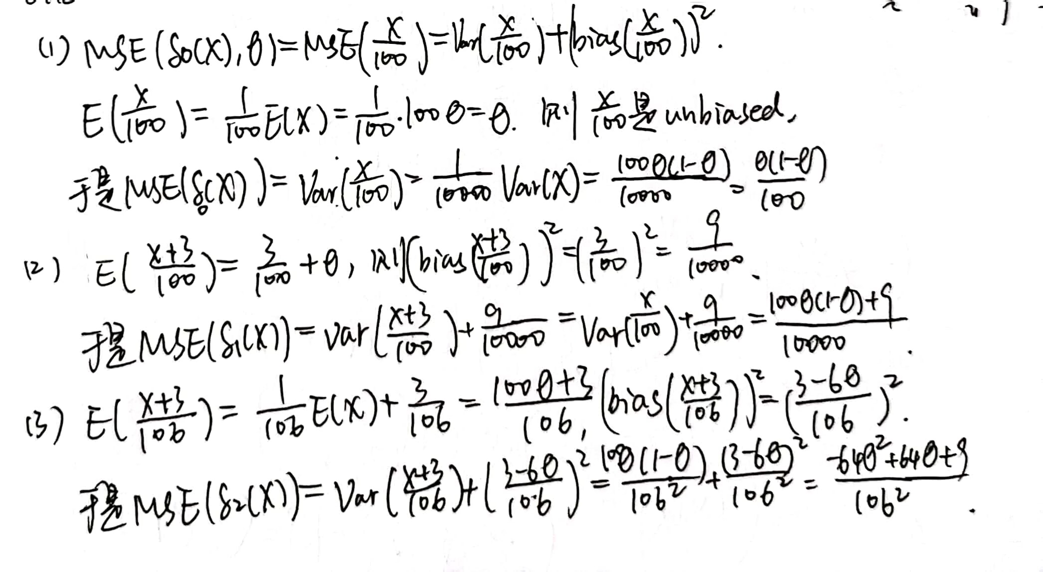
• Example 1：

  

  

  

  Example 2：

  

  

  

求估计量的方法——矩法

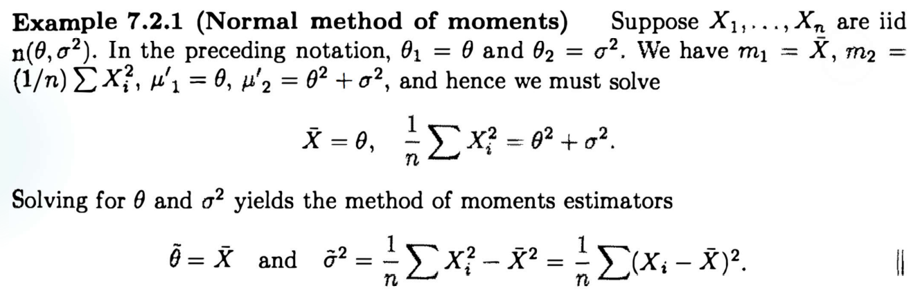
• \(X_1,X_2,...,X_n\) 是来自于以 \(f_\theta(x)\) 为 PDF 的有有限 \(k\) 阶矩的随机样本，\(\theta=(\theta_1,...,\theta _k) \in R^k\) 是未知的。定义：

  • Sample moment：\(m_1 = \frac{1}{n} \Sigma_{i=1} ^n X_i,m_2=\frac{1}{n}\Sigma_{i=1} ^n X_i^2,...\)
  • Population moment：\(\mu_1 = E(X_1)=h_1(\theta),\mu_2=E(X_1 ^2)=h_2(\theta),...\)

• Method of Moment（MOM）approach：对于未知的 \(\theta=(\theta_1,...,\theta_k)\)，可以通过求解 \(k\) 个方程 \(m_i=h_i(\theta)\) 来确定它们每个的 estimator，\(k\) 个方程确定 \(k\) 个“未知数”，很合理。

  事实上，这样解出来的 estimator 称为 moment estimator，也有可能解不出来。

• Example 1：

  

• 矩法得到的 moment estimator 不一定唯一，比如取前 \(k\) 个方程和取后 \(k\) 个方程得到的结果可能是不一样的，有很多例子。为了计算方便，我们尽量会取低阶矩。为了 unbiasedness，往往会取中心矩。

• MOM estimator 的性质：

  • 无偏性：样本原点矩一般都无偏，其余的没有一致的论断。

    

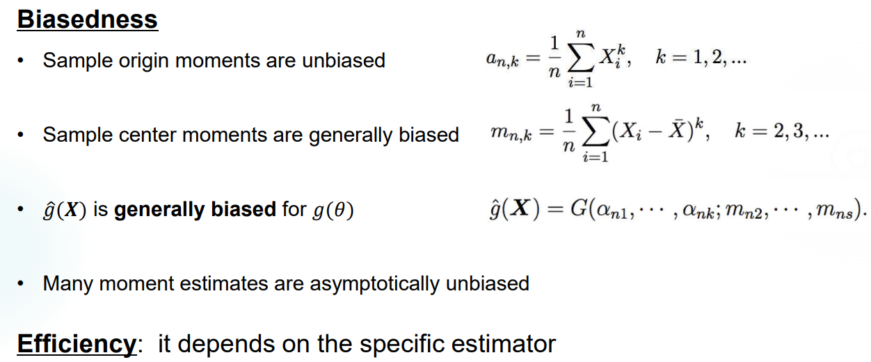
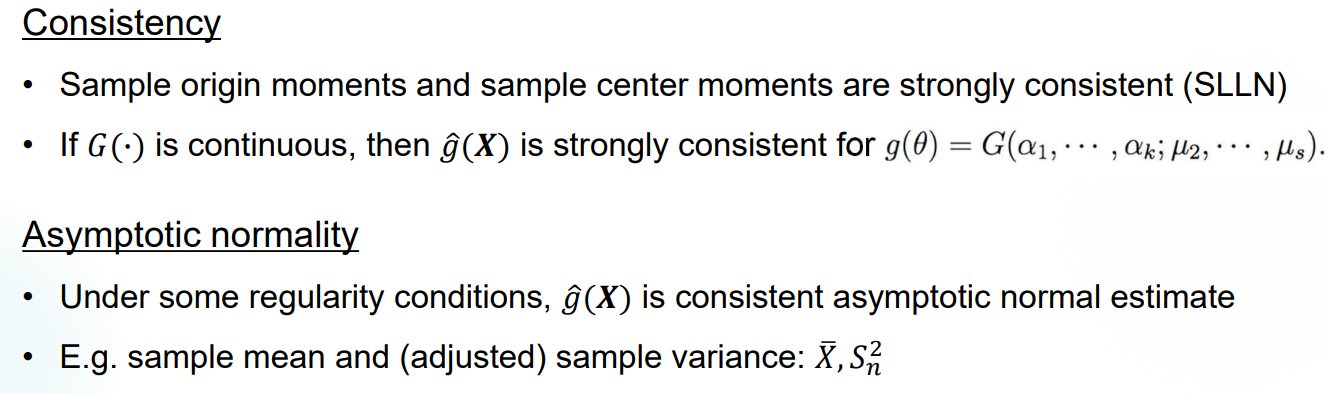
  • 相合性：

    

• MOM 的优缺点：

  • 简单好算，不用知道分布。
  • 样本较小时可能不精确，不一定完全反映样本的特征（漏参数）。

Homework 2

Lecture 5

本节介绍另一种点估计方法——Maximum Likelihood Estimator，这是最为流行的方法。

没想到的是这一讲还讲了一些数值方法，收敛到数值分析去了，我血赚（x

极大似然估计量 (MLE)

定义

• 找一个使得似然函数的值最大的常数 \(\theta\)，其函数作为一个 estimator，称为 maximum likelihood estimator。

• MLE 的求法不一定是求导，先看看求导能不能做 && 算出来的结果对了没有 && 有没有更简单的方法

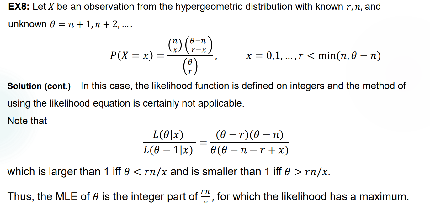
• 举个超几何分布的例子，这个问题的主要难度其实在于意识到，\(X\) 单点就是一个观测值，以及用离散方法。

  

性质

• Invariance Property：如果 \(\hat{\theta} _{MLE}\) 是 \(\theta\) 的 MLE，且 \(g\) 是任意的函数，则 \(g(\hat{\theta} _{MLE})\) 是 \(g(\theta)\) 的 MLE。

• Consistency：在某些条件下，MLE 序列依概率收敛到某个 \(\theta\) 值。（非常模糊，看看就好

• MLE & sufficient statistic：\(X=(X_1,X_2,...,X_n)\) 是 Population 中的一个随机抽样，Population 服从 \(\lbrace f(x;\theta),\theta \in \Theta \rbrace\) 的分布。如果 \(T=T(X_1,...,X_n)\) 是一个充分统计量，且 \(\theta\) 的 MLE 存在，那么 \(\hat{\theta}=\psi(T)\) 是 \(T\) 的一个函数。

• Asymptotic normality：在某些情况下，MLE \(\hat{\theta}\) 的序列（作为一个未赋值的随机变量）趋近于正态分布，准确来说，\(\sqrt{n} (\hat{\theta}_n - \theta) \to N(0,\sigma_\theta ^2),n\to \infty\)。其中，\(\sigma_\theta ^2 = \frac{1}{I(\theta)}\)，\(I(\theta)\) 是 \(X\) 的概率密度函数 \(f(x;\theta)\) 导出的 Fisher Information。

  如果使用 Delta Method，可以导出 \(\sqrt{n}[g(\hat{\theta}_n)-g(\theta)] \to N(0,(g'^2(\theta)/I(\theta)))\)。

  以上均为依分布收敛。

• 相比于矩法，MLE 方法有求解更快的优点，但有时缺乏数值稳定性，且必须知道 Population 的分布。

MLE 的数值解法

• 主要是使用牛顿法求解没有显式解的一阶微分方程。

MLE 的应用

• 标记重捕法：标记重捕过程实际上可以视为超几何分布过程，使用关于 \(\theta\) 的 MLE 估计即可。例如，第一次捉住了 10 只蜻蜓，全部做标记后放归。第二次捕捉 20 只蜻蜓后发现其中 4 只做了标记，希望求得种群数量 \(N\) 的估计值。实际上，记第二次捕获的蜻蜓里有 \(r\) 只做了标记，\(N\) 可以被视为随机变量 \(r\) 的分布中的参数，即 \(L(N;r)=f(r;N)=\frac{C_{10} ^r C_{N-10}^{20-r}}{C_N ^{20}}\)，得到 \(N\) 的 MLE 为 \(\hat{N}=[\frac{200}{r}]\)，种群总数为 50 只的概率最大。

• Hardy-Weinberg Law: 一个二倍体基因型包括两个基因，每个基因有两种表示，A 和 a。在人群中随机抽样得到 56 人中有 13 个为 AA 型，24 个为 Aa 型，19 个为 aa 型。求此基因显示为 A 的概率的 MLE。

  实际上可以将以上抽样视作对一个服从 \(B(112,\theta)\) 的 Population 进行抽样，得到一个容量为 112 的样本，其中抽取得到 50 个 A 和 62 个 a。考虑此样本的 Joint PDF 为 \(f(X)=C_{112} ^{50} \theta ^{50} (1-\theta) ^{62}\) 取最大值时，\(\theta=\frac{25}{56}\) 即为解。

Lecture 6

本节重新介绍 Fisher Information，并给出最后一种点估计方法——UMVUE。

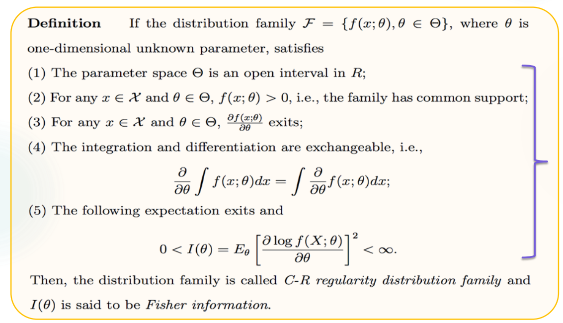
Regular Condition

一共有五条，分别提示了开集，概率密度为正，对参数的导数存在，对参数的求导和对 x 的积分可交换，Fisher Information 有限。

Revisit Fisher Information

• Random Sample 的 Fisher Information

  

• Population 的 Fisher Infomation

  

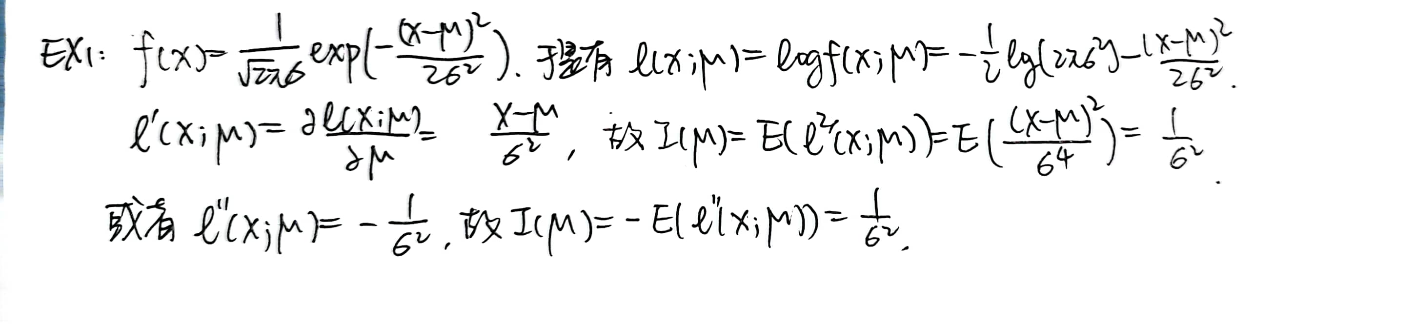
• Example 1：对于\(X\sim N(\mu,\sigma ^2), \sigma^2\) 已知，求 \(I(\mu)\)。

  

• 对于一个 estimator 序列 \(\lbrace \hat{\theta}_n \rbrace\)，有 \(\sqrt{n} (\hat{\theta}_n -\theta _0) \to N(0,\frac{1}{I(\theta _0)})\) 依分布收敛。考虑正态分布的性质可知，有 \(\hat{\theta}_n -\theta _0 \to N(0,\frac{1}{nI(\theta _0)})\)。其中 \(\theta_0\) 表示参数的真值。

UMVUE

定义

• The best unbiased estimator 是方差最小的无偏估计量，因此其 MSE 也最小。也可以指 UMVUE，也即 uniformly minimum variance unbiased estimator，一致最小方差无偏估计。其中的 uniformly 指的是对所有的参数都成立。

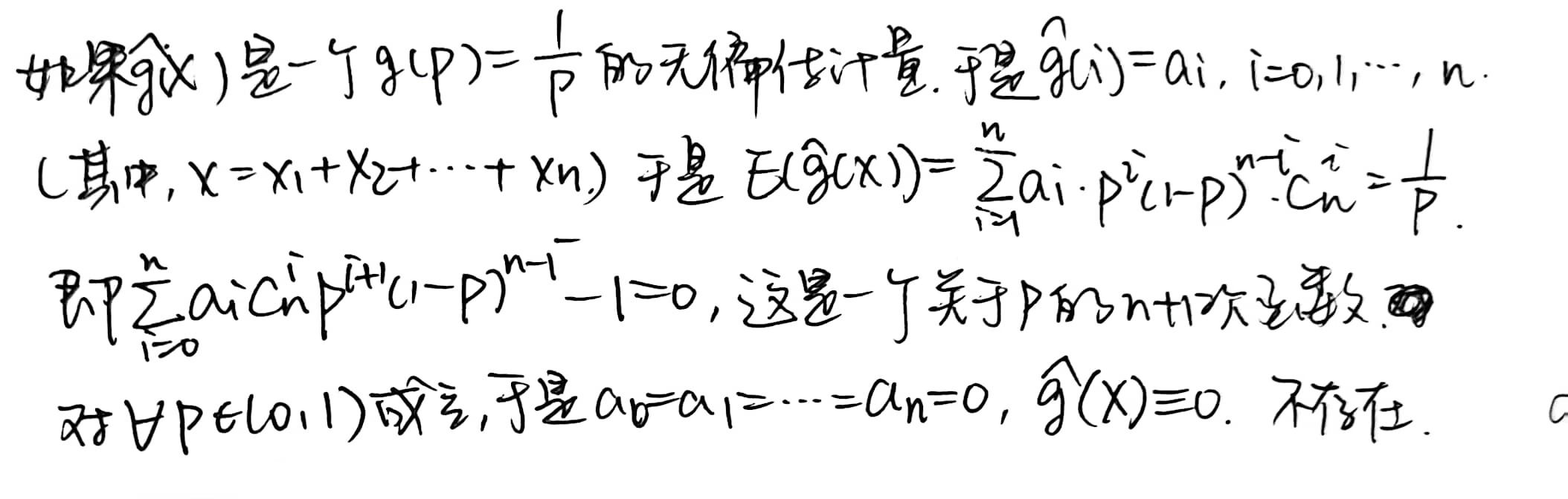
• 当然，一个样本可能不存在 unbiased estimator，也就没有 UMVUE，比如：

  \(X_1,X_2,...,X_n i.i.d. \sim B(1,p)\)，\(g(p)=\frac{1}{p}\) 是要进行估计的量，它没有无偏估计量。

  

• 每个无偏估计都是 sufficient estimator 的函数。

验证 UMVUE

• 对于随机抽样 \(X_1,X_2,...,X_n\)，样本对 \(\theta\) 的充分统计量为 \(T(X)\)，则 \(h(T(X))\) 是 UMVUE 当且仅当对任意 \(0\) 的无偏统计量 \(\psi(T(X))\)，有 \(cov(\psi(T(X)),h(T(X)))=0\)。其中有 \(E(\psi(T(X)))=0\)。

• Example 1：

  

寻找 UMVUE

寻找总比验证更困难。

• Cramer-Rao Inequality：\(X_1,X_2,...,X_n\) 是服从 PDF \(f(x | \theta)\) 的随机样本，\(W(X)=W(X_1,...,X_n)\) 是 \(X\) 的一个统计量，满足 \(\frac{d}{d\theta} E_\theta W(X) = \int \frac{\partial}{\partial \theta} [W(x)f(x|\theta)] dx\)，且 \(Var_\theta W(X) < \infty\)，于是 \(Var_\theta (W(X)) \geq \frac{(\frac{d}{d\theta} E_\theta W(X))^2}{nI(\theta)}\)。

  如果一个 unbiased estimator 达到了 C-R lower bound，它就是 UMVUE。然而这不是充要条件，任意一个 UMVUE 未必满足取等条件。且需要注意只有在满足 Regularity Conditions 的时候才能保持 Cramer-Rao 成立。

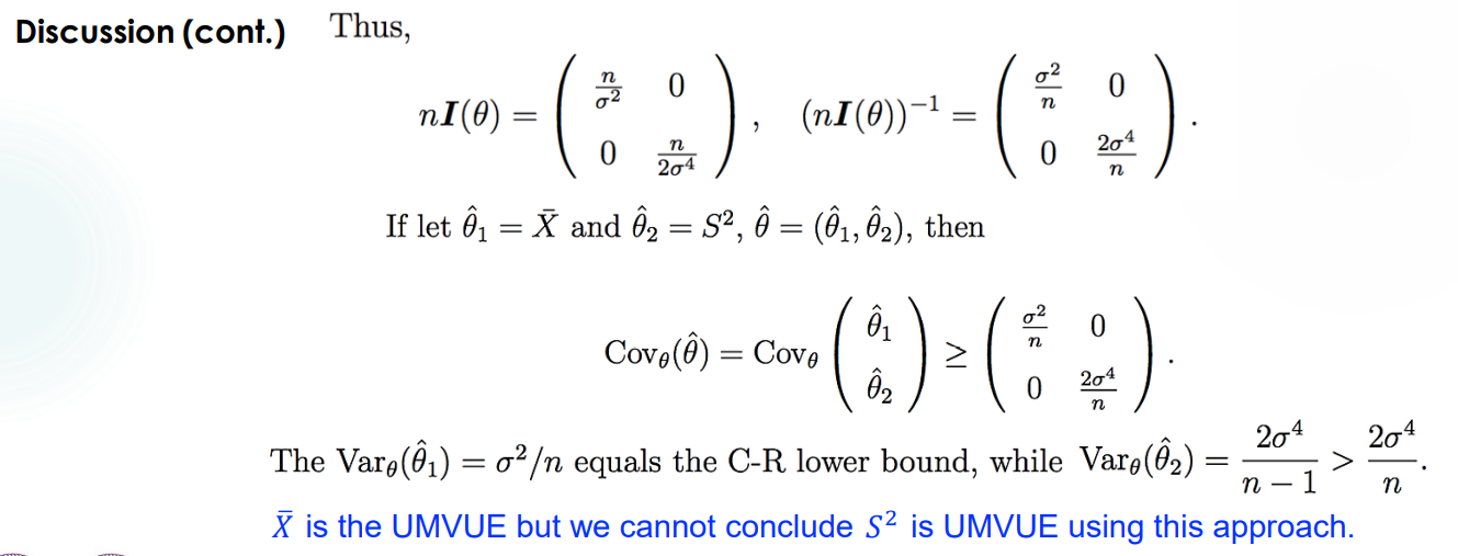
• 多元形式的 Cramer-Rao Inequality：\(Cov_\theta(\hat{\theta}) \geq (nI(\theta))^{-1}\)。其中，\(A\geq B\) 表示 \(A-B\) 是一个非负定矩阵。

• Example 1：

  

  

• Rao-Blackwell：\(T(X)\) 是 \(g(\theta)\) 的 sufficient statistic，\(\hat{g}(X)\) 是 \(g(\theta)\) 的 unbiased estimator，于是记 \(h(T)=E(\hat{g}(X)|T)\) 也是一个 unbiased estimator，且 \(Var(h(T))\leq Var(\hat{g}(X))\)。

  这是一个把 unbiased estimator 的方差降低的方法，启发出以下的 Lehmann-Scheffe Theorem。

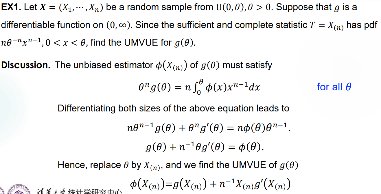
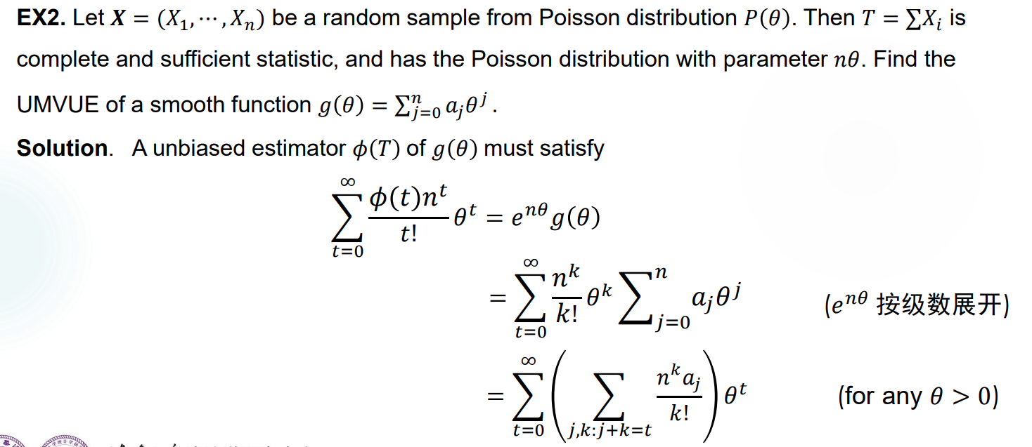
• \(T(X)\) 是 \(g(\theta)\) 的 complete and sufficient statistic，如果 \(\hat{g}(T(X))\) 是 unbiased estimator，那么它就是唯一的 UMVUE。

• \(T(X)\) 是 \(g(\theta)\) 的 complete and sufficient statistic，\(U\) 是 \(g(\theta)\) 的 unbiased estimator，那么 \(\hat{g}(T)=E_\theta (U|T)\) 也是唯一的 UMVUE。

  这给出了已知 complete and sufficient estimator 时的两种方法：要么直接寻找其函数使得它也是 unbiased estimator，要么得到一个 unbiased estimator 然后二者结合做出解。显然，对于 Exponential Family 中的分布来说，这个方法比较容易操作，因为我们可以轻松地找到 complete and sufficient estimator。

  注意一个特例：Normal Distribution 的 UMVUE 就是对应的 \(\bar{X},S^2\) 在系数和常数上的修正，这是易于证明的。

• Example 1：

  

• Example 2：

  

  

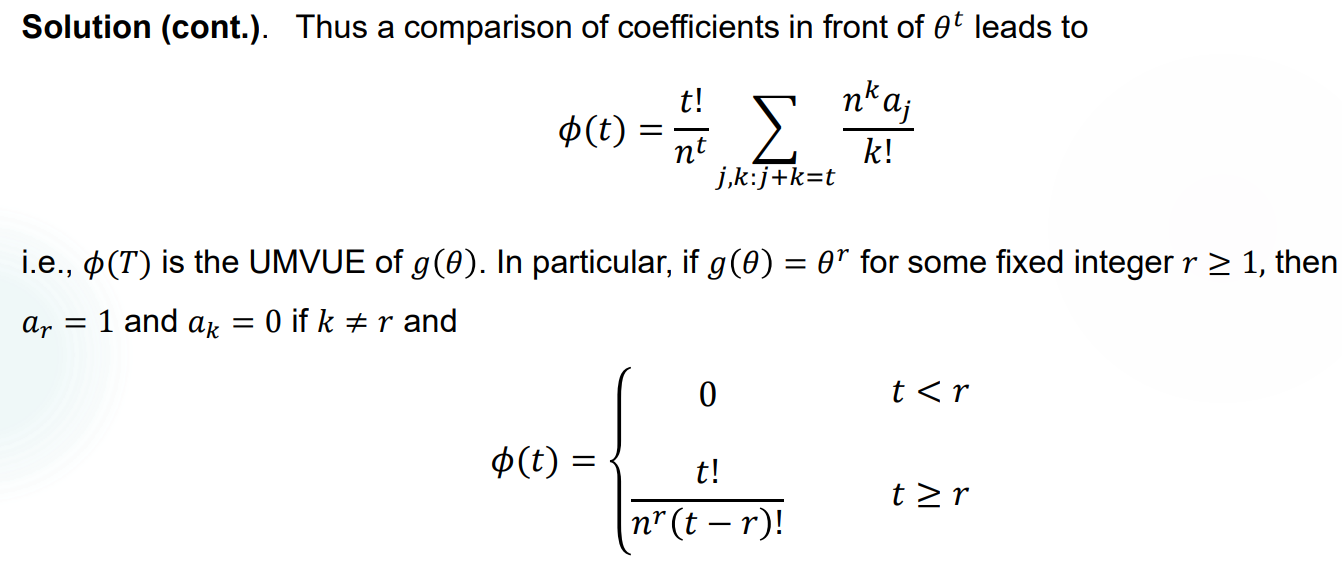
• Example 3：

  

判别无偏统计量的有效性

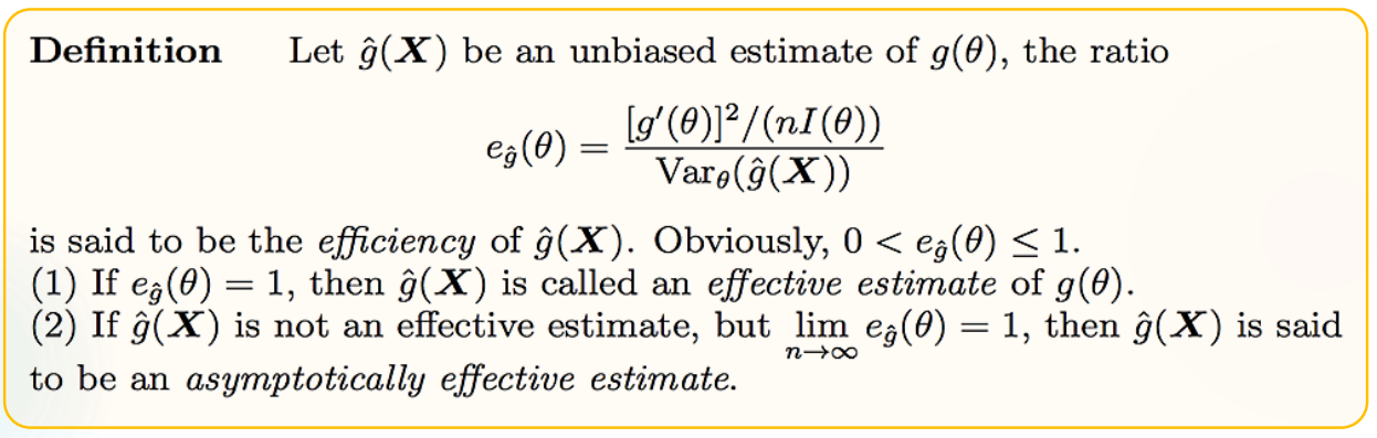
• Efficiency：

  

Homework 3

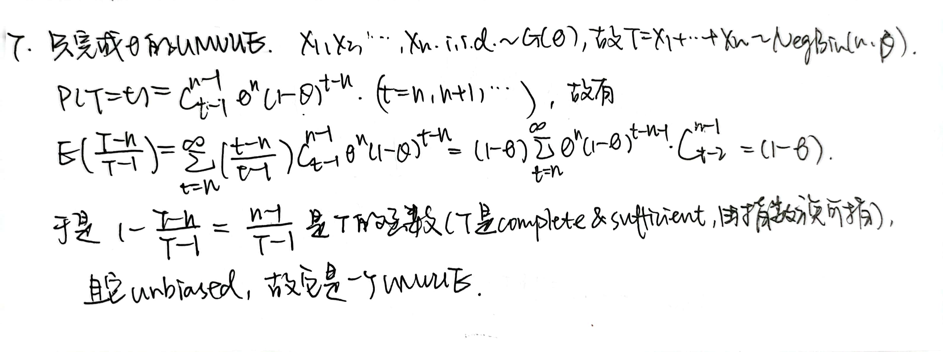
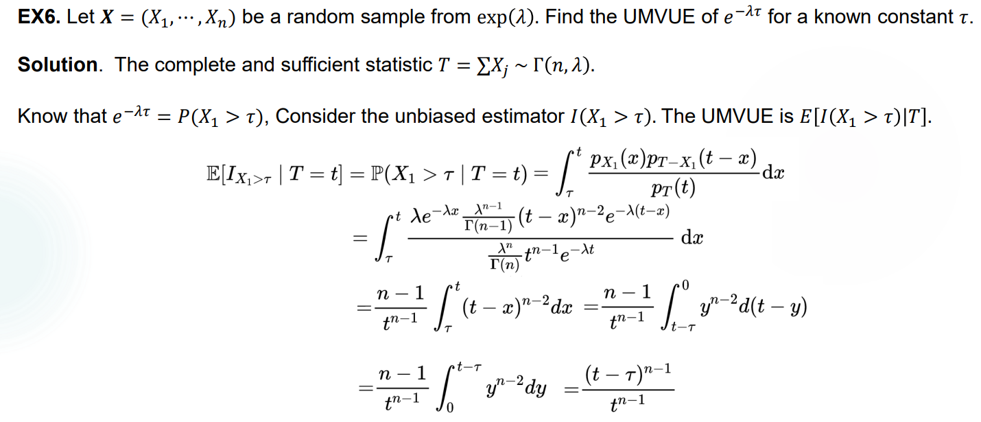
后记：期中考试又考了一遍这个题，不过问的是 \(\theta ^2\) 的 UMVUE。考场上自己写的时候才发现根本不用这么复杂，在第三行那一步的时候凑一个 \(\theta ^2\)（此处是 \(\theta\)）出来就行，搞不懂助教为什么凑的是 \(1-\theta\)。结果是一样的，毕竟用 complete & sufficient statistic 得出的 UMVUE 是唯一的。

\(\theta ^2\) 的 UMVUE 是 \(\frac{(n-1)(n-2)}{(T-1)(T-2)}\)，可见与 \(\theta\) 的 UMVUE 形式类似。

Mid-Term

Click Here

问就是，不是我写的，跟我没关系，请不要开盒.jpg

Lecture 7

本节介绍区间估计，它对于参数的估计就更模糊一些，注重于根据一系列数据来提供若干个区间，使得参数的函数值落在其中。听起来没那么完美，但是现实就是这样的嘛。

Interval Estimation

定义

• 任意的 statistic \(\hat{g}_1(X),\hat{g}_2(X)\) 满足 \(\hat{g}_1(X) \leq \hat{g} _2 (X)\)，则区间 \([\hat{g}_1(X),\hat{g}_2(X)]\) 是 \(g(\theta)\) 的一个 interval estimate（也可以叫做 confidence interval）。这个定义很宽泛，因为一个区间估计未必需要 \(g(\theta)\) 落在其中，它可以是无效的。需要注意的是，此处的用词是 estimate，意思是说，这里的 \(X\) 指的是一个确切的样本。

• coverage probability：区间 \([\hat{g}_1(X),\hat{g}_2(X)]\) 的 coverage probability 是随机区间 \([\hat{g}_1(X),\hat{g}_2(X)]\) 包括真实值 \(g(X)\) 的概率，也就是 \(P\lbrace g(\theta) \in [\hat{g}_1(X),\hat{g}_2(X)] \rbrace >0\)。

• Example 1：

  

  

Measurement

然后就是要衡量一个 interval estimation 的有效度。

• \(X_1,X_2,...,X_n\) 是一个服从 \(f(x;\theta)\) 的随机样本。Confidence Level（置信度，也写作 reliability）被定义为 \(P(\theta \in [\hat{\theta_1},\hat{\theta_2}])=P(\hat{\theta_1}\leq \theta \leq \hat{\theta_2})\)。

• Confidence coefficient（置信系数）：\(inf_{\theta \in \Theta} P_\theta (\hat{\theta _1} \leq \theta \leq \hat{\theta_2})\)

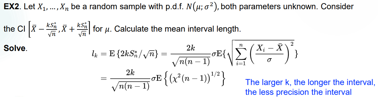
• Precision（精确度）：有很多种估计方法，此处取最常用的方法：mean interval length，即计算 \(E_{\theta}(\hat{\theta_2}-\hat{\theta _1})\)，这个值越大说明区间越长，因此估计的精确度越差。

  一般来说，置信度和精确度是一对相反的要求，需要进行 trade-off。

• Example 1：

  

• Revisit Confidence Interval：重新对于 confidence interval 进行定义，加上 confidence coefficient 的条件后如下：区间 \([\hat{\theta _1}(X),\hat{\theta _2}(X)]\) 是 \(\theta\) 的一个 interval estimate，且对于一个给定的 \(\alpha\) 有 \(0<\alpha <1\)，如果 \(P(\hat{\theta_1}(X)\leq \theta \leq \hat{\theta_2}(X)) \geq 1-\alpha\)，那么称区间 \([\hat{\theta _1}(X),\hat{\theta _2}(X)]\) 是一个有 confidence level 为 \(1-\alpha\) 的， \(\theta\) 的 confidence interval。

  于是 confidence coefficient \(inf_{\theta \in \Theta} P_\theta (\hat{\theta _1} (X)\leq \theta \leq \hat{\theta_2}(X)) \leq \alpha\)，是 confidence interval \([\hat{\theta _1}(X),\hat{\theta _2}(X)]\) 的 confidence coefficient。

• Remark 1：此处如果有 \(\alpha=0.05\)，不代表 \(\theta\) 有 \(0.95\) 的概率落在得到的区间里，而是指的是我们有 \(0.95\) 的信度能够确定 \(\theta\) 在此区间里。更形象地，我们取 \(1000\) 个样本，得到的 \(1000\) 个区间里大约会有 \(950\) 个覆盖住 \(\theta\)。

• Remark 2：在取样本之前，所有的区间 \([\hat{\theta _1}(X),\hat{\theta _2}(X)]\) 都是 random interval，但取得样本之后区间的左右端都变为定值，称为 observed interval。

• Confidence Limit：有的时候我们只关心参数的上界或下界，即只考虑单边。对于给定的 statistic \(\hat{\theta}_U (X),\hat{\theta}_L (X)\)，对于给定的 \(0<\alpha <1\)，如果 \(P_\theta(\theta \leq \hat{\theta}_U (X))\geq 1-\alpha,\theta \in \Theta\)，或者 \(P_\theta(\theta \geq \hat{\theta}_L (X))\geq 1-\alpha,\theta \in \Theta\)，则称 \(\hat{\theta}_U (X),\hat{\theta}_L (X)\) 分别是 \(\theta\) 的 upper confidence limit 和 lower confidence limit，且有置信度 \(1-\alpha\)。

  针对 confidence limit 的 precision 估计：\(E(\hat{\theta}_U(X))\) 越小或者 \(E(\hat{\theta}_L(X))\) 越大，越精确。

  此时，取 confidence interval 为 \([\hat{\theta _L}(X),\hat{\theta _U}(X)]\)，它的 confidence level 为 \(1-\alpha_1-\alpha_2\)。

多维情形

略（

构造合适的 Interval Estimation

Pivot quantity method

如果要翻译的话，可以称为“枢轴量方法”。

• 寻找 Pivot Quantity 的方法：找到一个包含参数 \(\theta\) 的随机变量，它关于 \(X_1,X_2,...,X_n\) 的部分最好是一个充分统计量的形式，且这个随机变量的分布已知。

  观察此 pivot quantity 落在区间 \([a,b]\) 上的概率，并适当选取让这个概率大于 \(1-\alpha\)。

  再把这个式子改成关于 \(\theta\) 的 interval estimation 的形式。

• 总之，要找一个分布与 \(\theta\) 无关，且形式上与 \(\theta\) 有关的随机变量，它在形式上也不能和其他未知的参数有关。

• 位置-尺度族的常用 Pivot Quantity：

  Form of PDF	Type of PDF	Pivotal Quantity
  \(f(x-\mu)\)	Location	\(\bar{X}-\mu\)
  \((1/\sigma)f(x/\sigma)\)	Scale	\(\bar{X}/\sigma\)
  \((1/\sigma)f((x-\mu)/\sigma)\)	Location-Scale	\((\bar{X}-\mu)/S\)

Approximate CI

• 顾名思义，在找不到合适的 pivot estimation 的时候，可以利用中心极限定理等方式取得一个依分布收敛的随机变量，把它作为 pivot estimation，然后进行考虑。

• 常用于不确定分布的 Population，或者无法求得合适的 pivot estimation 的 Population。如果有精确的 pivot estimation 但是转化为参数中心的不等式时计算太复杂，也可以将其中的项进行改动，比如把某个 \(\mu\) 改成 \(\bar{X}\)，等等。

• Example 1：

  

• 前提是样本量足够大。

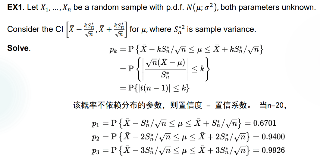
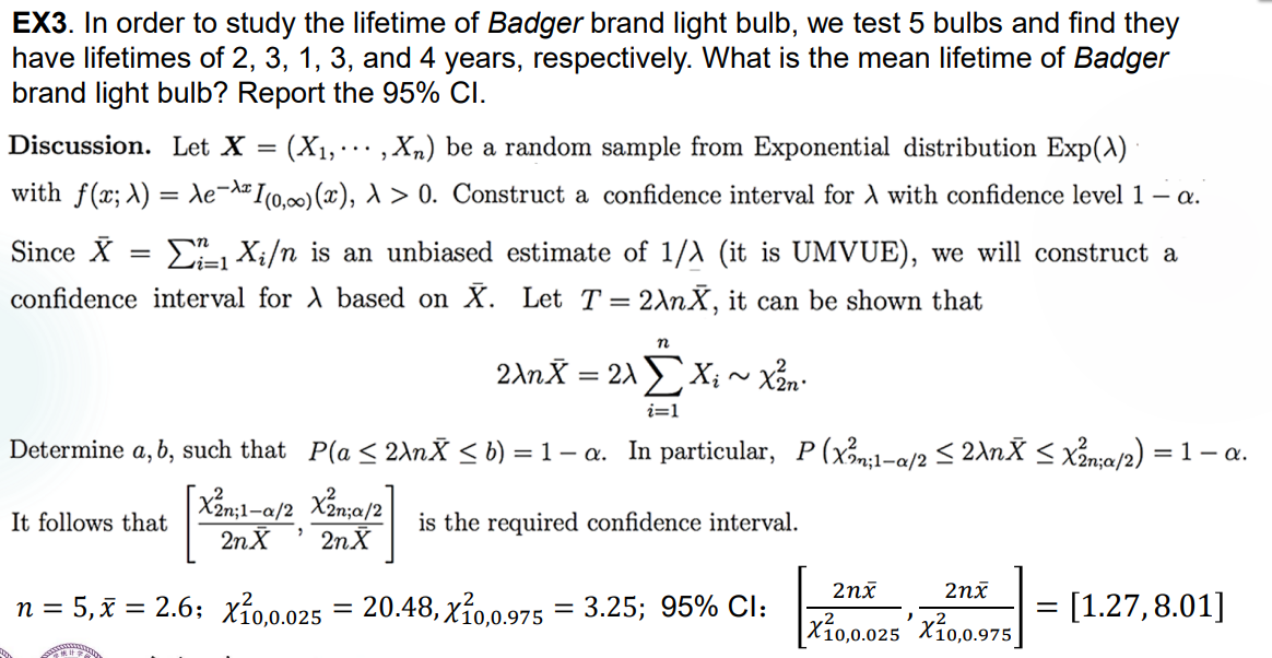
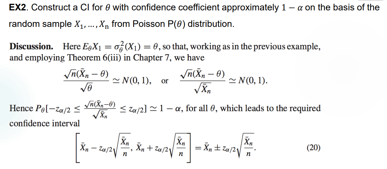
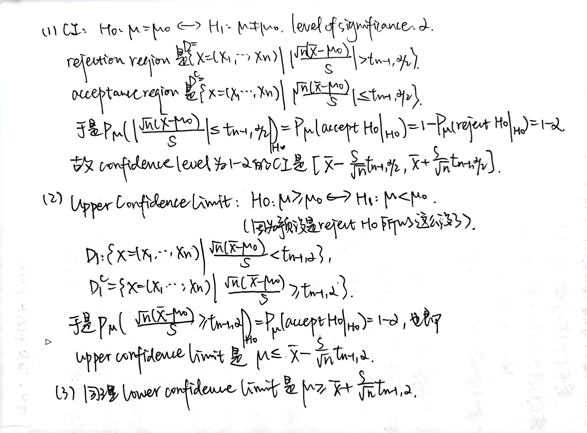
关于正态分布的 CI

幸运的是，下面这张图上有你需要的一切：

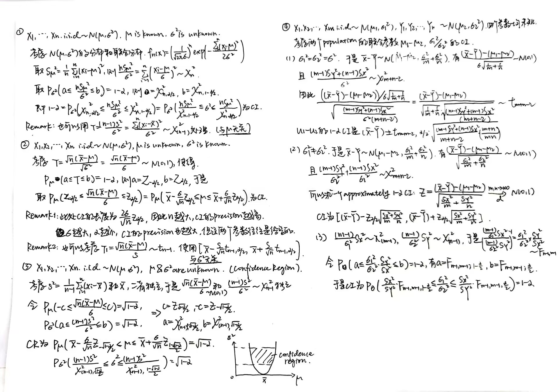
• 1 和 2 指出的是对于某个随机样本 \(X_1,...,X_n i.i.d \sim N(\mu, \sigma^2)\)，在参数之一已知的时候，求出另一参数的 CI 的方法。在 Remark 里提出了不需要已知参数时的方法。

• 3 指出的是两个参数都不可知时，利用独立性得出 \(\mu,\sigma^2\) 的 Confidence Region 的方式，虽然考试中并不会涉及，但是我觉得思路相当好。

• 4 指出的是两个不同的正态 Population 中分别取样，得出 \(\mu_1-\mu_2\)，\(\frac{\sigma_1 ^2}{\sigma_2 ^2}\) 的 CI 的方法。

  分类讨论了几种：在方差相等时 \(\mu_1-\mu_2\) 的 CI 可以准确求出（如果已知了 \(\sigma\) 甚至更方便，用标准化到正态分布的 \(T\) 就可以做了），方差不等时 \(\mu_1-\mu_2\) 的 CI 是 approximate 的；此外，\(\frac{\sigma_1 ^2}{\sigma_2 ^2}\) 的 CI 求法在最后一种情况里给出。

Homework 4

略，基本就是以上内容的简单应用，不过计算量有点大（

Lecture 8

心情如图所示：orz orz orz orz orz orz

本节介绍假设检验的一些基本信息，这也是直到学期末为止的后半部分课程的主要内容。

突然想起 V1ncent19 学长说过的一段话：

如果对生存分析不太熟悉的同学可以先笼统地理解为研究“某件事情什么时候发生”，这个时候就不得不提起某蒙古上单的评论“* * 什么时候 * 啊”，大概就是研究这种事情。

所以假设检验的通俗解释大概就是，对于某个样本，我们先验证它是否满足 A 条件，如果满足，我们就认为某个与参数相关的结论 B 是对的。否则，有一个和结论 B 矛盾的结论 C 成立。生活中其实处处都是假设检验，类似于通过“今天 ta 和我说话了”来判断出“ta 一定喜欢我吧！”这一假设成立，显然信度不是很高。

基本定义

检验的定义

• Hypothesis Testing：我们有一个 distribution family 为 \(F=\lbrace f(x;\theta),\theta \in \Theta \rbrace\)，记 \(X=(X_1,X_2,...,X_n)\) 是上述分布族中的一个随机样本。记 \(\Theta_0\) 是 \(\Theta\) 中不为空的一个子集，我们想检验是否有 \(\theta \in \Theta_0\)。记 \(\Theta_1=\Theta - \Theta_0\) 是 \(\Theta_0\) 的补集。

  • Null Hypothesis（原假设）：记为 \(H_0\)：\(\theta \in \Theta_0\)，说明存在某个 \(\theta_0 \in \Theta_0\)，使得 \(X_i \sim f(x;\theta_0)\)。
  • Alternative Hypothesis（备择假设）：\(H_0\) 的 Alternative Hypothesis 记为 \(H_1\)：\(\theta \in \Theta_1\)。
  • 于是假设检验过程可以写为：\(H_o:\theta \in \Theta_0 \leftrightarrow H_1 : \theta \in \Theta_1\)。
  • Simple and composite hypothesis ：\(H_0 (/ H_1)\) 是一个 simple hypothesis 等价于 \(\Theta_0(/ \Theta_1)\) 是一个单点集，否则是 composite hypothesis。

  根据样本检验 \(H_0\) 是否正确的过程，称作对于 \(H_1\) 检验假设 \(H_0\)。（我瞎翻译的，原文是 testing the hypothesis \(H_0\) against the alternative \(H_1\)）

  在 Hypothesis Testing 中，null hypothesis \(H_0\) 称为 original belief，是一个我们希望通过样本验证它是错的的精确条件。我们一般预设它是错的，预设 alternative hypothesis 是对的。

• Rejection Region：在一个随机样本 \(X=(X_1,X_2,...,X_n)\) 上我们要做出一个决定，即接受还是拒绝 null hypothesis \(H_0\)。也就是说我们要定义出一个条件 \(A\)，满足此条件则 accept null hypothesis，否则 reject null hypothesis。

  不满足条件 \(A\) 的样本 \(X\) 会使得 null hypothesis 被拒绝，符合我们的预设，这样的 \(X\) 的集合称为 Rejection Region（或称 critical region），记为 \(D\)，是一个样本子空间。于是 \(D^c\) 就是 Acceptance Region，满足 \(\chi=D+D^c\)，\(\chi\) 是样本空间。

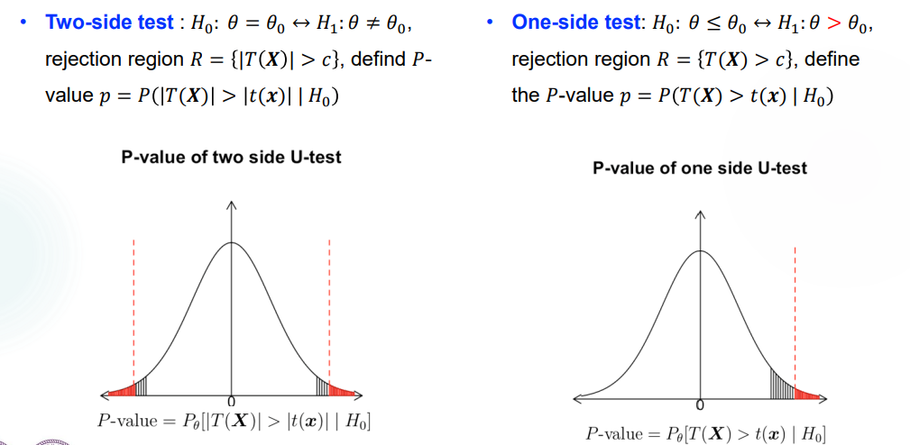
• Two-side 和 One-side test：

  • 双边检验：\(H_0:\theta=\theta_0 \leftrightarrow H_1:\theta \neq \theta_0\)，它的检验条件 \(A\) 是 \(A: -c \leq T(X)\leq c\)，其中 \(T(X)\) 是 \(\theta\) 的一个估计量。于是 rejection region 就是 \(D=\lbrace |T(X)| >c \rbrace\)。

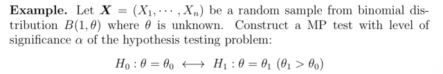
  • 单边检验：\(H_0:\theta \leq \theta_0 \leftrightarrow H_1 : \theta > \theta_0\)，它的检验条件 \(A\) 是 \(A: T(X)\leq c\)，其中 \(T(X)\) 是 \(\theta\) 的一个估计量。于是 rejection region 就是 \(D=\lbrace T(X) >c \rbrace\)。

    对称地，如果 \(H_0:\theta \geq \theta_0 \leftrightarrow H_1 : \theta < \theta_0\)，它的检验条件 \(A\) 是 \(A: T(X)\geq c\)，其中 \(T(X)\) 是 \(\theta\) 的一个估计量。于是 rejection region 就是 \(D=\lbrace T(X) <c \rbrace\)。

检验函数

• Test Function：在某些非黑即白的检验条件下，\(\psi(X)=I_{\lbrace reject H_0 \rbrace}\)。也就是说 \(H_0\) 被 reject、符合预设的时候 test function 取为 \(1\)，否则取为 \(0\)。

  实际上，更标准的 test function 定义为 reject \(H_0\) 的概率，如果是 non-randomized test 则 \(\psi(X)=0,1\)，如果是 randomized test 则 \(\psi(X)\) 可取 \([0,1]\) 之间的值。

• 以下考虑一些 randomized test。

  Example 1：

  

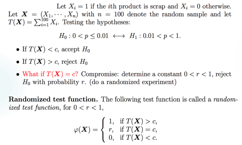
  由此定义 randomized test function：临界条件下定义 \(\psi (X)=r\)，\(X\in D\) 时 \(\psi(X)=1\)，否则 \(X\in D^c\) 时 \(\psi (X)=0\)。

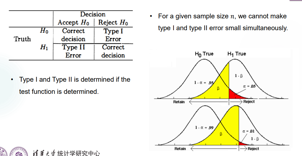
Type I & II Errors

实际上，我们在假设检验中进行随机抽样，总有可能取到偏误的样本，导致错误地 reject 或者 accept 了 \(H_0\)。有两种错误，分别称为 Type I & II Error。

• 通俗来说，Type I Error 是假阳性，也就是把实际正确的 \(H_0\) 给 reject 了，就像给健康人判了感染一样。发生 Type I Error 是因为取到的样本恰好落在了 \(D\) 里，这个概率是：

  \(\alpha(\theta)=P(I)=P[(X_1,X_2,...,X_n) \in D | H_0]=P[(X_1,X_2,...,X_n) \in D | \theta \in \Theta_0]\)

  发生 Type I Error 的最大概率，也就是 \(\alpha=max_{\theta \in \Theta_0} P(I)\)，称为 the level of significance（显著性水平）。当 \(\alpha=0\) 时说明 \(D=\emptyset\)，也就是说 \(H_0\) 永远被接受。

• 相对地，Type II Error 就是假阴性，\(P(II)=P[(X_1,X_2,...,X_n) \in D^c | \theta \notin \Theta_0]\)。

  定义发生 Type II Error 的概率为 \(\beta(\theta)\)，于是 \(\beta(\theta)=1\) 时也有 \(D=\emptyset\)，这是和预设不符的。

• 同时降低两种 Error 是不太可能的，以一个正态的估计量 \(T(X)\) 为例，可以看到呈一个此消彼长的趋势。（课上这个图画了好久，不是很懂，摸鱼去了）

  

  但是在实际操作中我们会遵循 Neyman-Pearson Principle，去尽量降低发生 Type I Error 的概率，让 the level of significance 降低到一个预设的级别 \(\alpha\)，再去考虑降低 Type II Error 的概率。

  于是如果样本落进了 \(H_0\) 的 acceptance region，我们会保持自己的预设，优先考虑这个样本没有提供足够的证据来 reject \(H_0\)，而不是我们应该 accept \(H_0\)。

Power Function

• Power Function（功效函数，势函数）定义为一个假设检验中，样本落在 \(H_0\) 的 rejection region \(D\) 上的概率，即 \(\pi(\theta)=P_\theta (X \in D)\)。当 accept \(H_0\) 时，\(\pi(\theta)=\alpha(\theta)\)，否则 \(\pi(\theta)=1-\beta(\theta)\)。

• 单次检验 \(\psi\) 的 power function 定义为 \(\pi_\psi(\theta)=E_\theta [\psi(X)]\)，其中 \(\psi(X)\) 是 reject \(H_0\) 的概率，也就是说 power function 是整个检验中 reject \(H_0\) 的概率总和。

  对于一个 non-randomized test，\(\pi_\psi(\theta)=P_\theta (X=(X_1,...,X_n) \in D)\)，因为 \(\psi\) 取值为 \(0,1\)。

  对于一个 randomized test，\(\pi_\psi(\theta)=P(T(X)>c)+rP(T(X)=c)\)，因为 \(\psi\) 取值 \(0,1,r\)。

• Example 1：

  

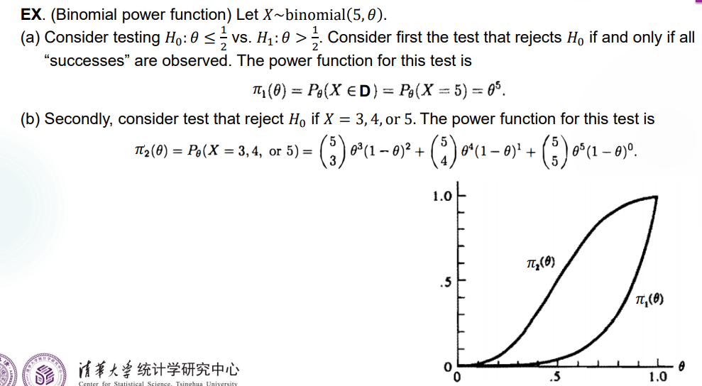
  Remark：这个题给出了两个 power function 的曲线，可以看到 \(\pi_1(\theta)\) 底部和 \(\theta\) 轴贴得比较近，对于 Type I Error 的预防较好；在 \(\theta\) 落在 \(\Theta_1\) 中时 \(\pi(\theta)=1-\beta(\theta)\)，因此 \(\pi_2(\theta)\) 对 Type II Error 的预防较好。

  实际上，这两个检验方式都不够好，没有同时预防两种 Error。最理想的 power function 应该在 \(\theta=0.5\) 处陡然上升，这样 \(\alpha(\theta)\) 和 \(\beta (\theta)\)，也即发生 Type I & II Error 的概率都能得到控制。

P-value

• 感觉不是很好理解，先举个例子。我们已经知道在假设检验的时候一般都有一个范围，例如在 \(T(X)>a\) 时 reject \(H_0\)，等等。当拿到一个样本计算出 \(T(X)\) 后，它在大于 \(a\) 时可能离 \(a\) 很远，也可能离 \(a\) 很近。离 \(a\) 越远，我们越确信这个样本更好地反映了应该 reject \(H_0\)。因此，我们希望找一个标准来衡量这种“确信”的程度，因此引入 P-value。

• 某一个样本 \(X\) 的 P-value 反映出了在 reject or accept \(H_0\) 这件事上有相同结果的时候，所能得到的其他样本比 \(X\) 更加极端的概率。虽然听起来很奇怪，但就是这样的。反映到具体例子里，大概就是：

  

  P-value 是一个基于所得样本的条件概率，前提是 \(H_0\) 成立。

• Decision Rule：给出一个衡量标准 \(\alpha\)，我们在 \(T(X)\) 符合判断要求，且 \(P-value \leq \alpha\) 时 reject \(H_0\)。因此，P-value 能够衡量做出 rejection of a hypothesis 这一决定的证据充分程度，P-value 越小，拒绝的理由越充分，这样的操作就可以称为一个 strong rejection，称结果 highly statistically significant（统计学上有高度的显著意义（我瞎翻译的

• Example 1（HW）：

  

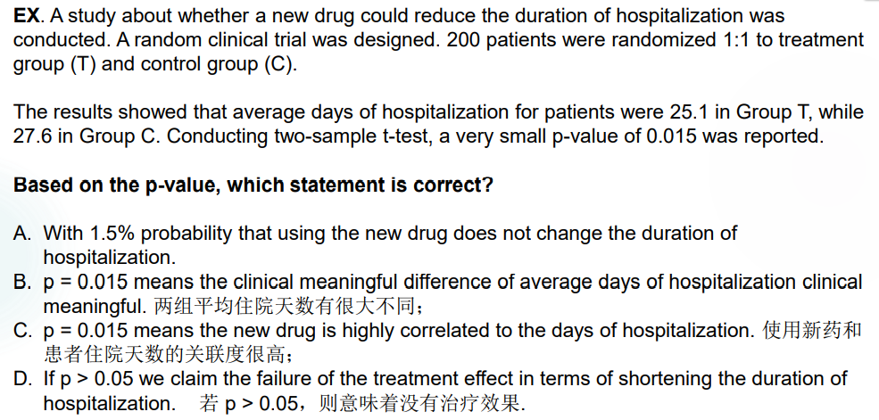
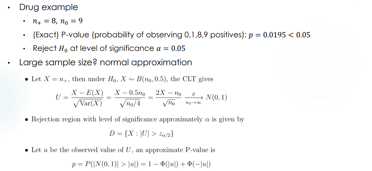
  先建个模：试验得到的样本是 \((x_1,x_2)=(25.1,27.6)\)，null hypothesis 指的是“药是无效的”，alternative hypothesis 指的是“药是有效的”（对此区分是因为我们预设 reject null hypothesis）。如今得到了一个比较小的 P-value 是 \(0.015\)，这说明了我们有比较大的把握通过这一个样本来确定药是有效的。

  四个选项都不对。\(A\) 选项计算的是 \(P(H_0)\)，\(B\) 选项计算的或许是 \(E(X_1-X_2)\)，\(C\) 选项计算的是 \(P(T(X_1)<a | H_0)\)，虽然在形式上比较接近 P-value 的定义了但还是不对，\(D\) 选项问题在于 \(p>0.05\) 时说明这一组样本对于 reject \(H_0\) 的可信度不够高，并不完全证明没有治疗效果。

• The American Statistical Association's statement on p-values: context, process, and purpose

  因为 P-value 真的很容易被误用，所以 ASA 在 2016 年提出了使用和解释 P-value 的原则。摘录如下：

  • P-values can indicate how incompatible the data are with a specified statistical model.

    A p-value provides one approach to summarizing the incompatibility between a particular set of data and a proposed model for the data.

    The smaller the p-value, the greater the statistical incompatibility of the data with the null hypothesis, if the underlying assumptions used to calculate the p-value hold.

  • P-values do not measure the probability that the studied hypothesis is true, or the probability that the data were produced by random chance alone.

    Researchers often wish to turn a p-value into a statement about the truth of a null hypothesis, or about the probability that random chance produced the observed data. The p-value is neither.

  • Scientific conclusions and business or policy decisions should not be based only on whether a p-value passes a specific threshold.

  • Proper inference requires full reporting and transparency.

  • A p-value, or statistical significance, does not measure the size of an effect or the importance of a result.

    Smaller p-values do not necessarily imply the presence of larger or more important effects, and larger p-values do not imply a lack of importance or even lack of effect.

    Any effect, no matter how tiny, can produce a small p-value if the sample size or measurement precision is high enough, and large effects may produce unimpressive p-values if the sample size is small or measurements are imprecise.

    Similarly, identical estimated effects will have different p-values if the precision of the estimates differs.

    (讲了一些选取 estimator 会带来的区别，课程还没涉及到)

  • By itself, a p-value does not provide a good measure of evidence regarding a model or hypothesis.

    Researchers should recognize that a p-value without context or other evidence provides limited information.

    For example, a p-value near 0.05 taken by itself offers only weak evidence against the null hypothesis.

  总的来说，P-value 能够提供的信息是有限的。

Lecture 9

本节继续介绍了以正态分布样本为主的假设检验。变得越来越像 Interval Estimation 了。

首先回顾一下假设检验的过程：

• 先设出一个 null hypothesis \(H_0\) 和对应的 alternative hypothesis \(H_1\)，二者不一定构成全集。
• 找到用于假设检验的 test statistic \(T(X)\)，以及对应的 rejection region \(D\)，例如 \(D=\lbrace X | T(X)>a \rbrace\)，\(a\) 是待定的。
• 找到一个合适的 level of significance \(\alpha\)，一般是 \(0.01,0.05\)，通过控制 critical value，也就是控制发生 Type I Error 的概率小于 \(\alpha\)，来决定 \(D\) 的具体形式。
• 取样本，计算 \(T(X)\)，看它是否在 rejection region 里，判断是否要 reject null hypothesis。
• 计算 P-value 的大小，来判断通过这组样本作出决定的这一做法有多大的可信度。

每一步都比较清楚了，目前落实到具体问题里需要处理的是找 test statistic，以及控制 critical value 来得到 rejection region 两步。

Testing in various populations

懒得翻译了，总之在正态分布的一些情况里、以及一些简单分布中进行分析。

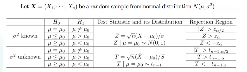
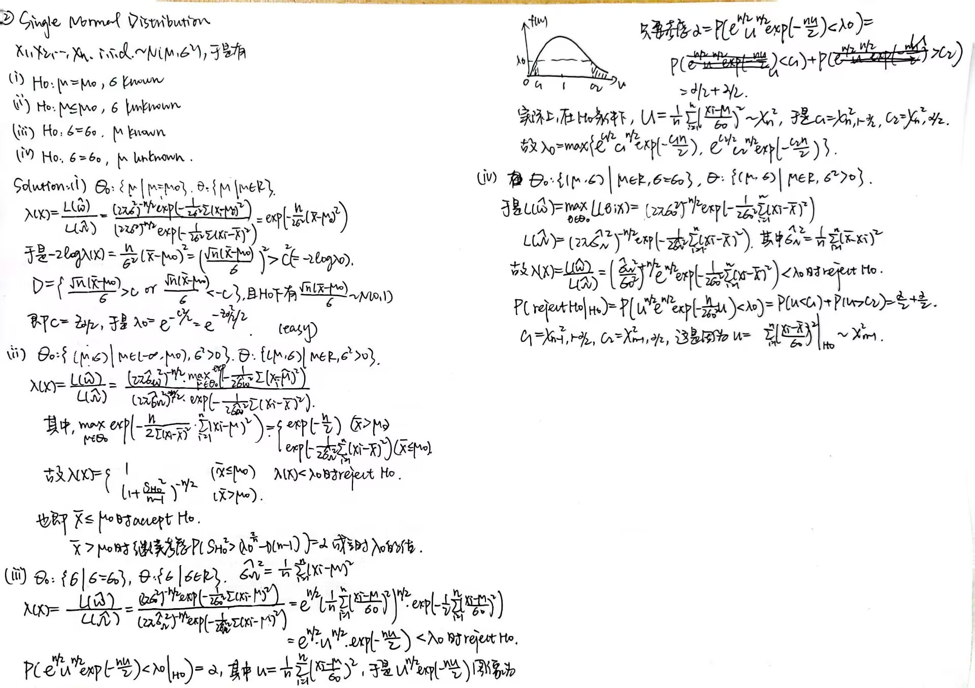
A single normal population

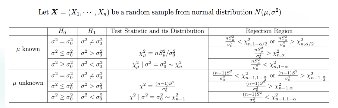
• 检验 \(\mu\) 的过程分为是否知道 \(\sigma\) 具体值的两种情况，又分为三种典型的 Hypothesis 进行处理，一切都在图中：

  

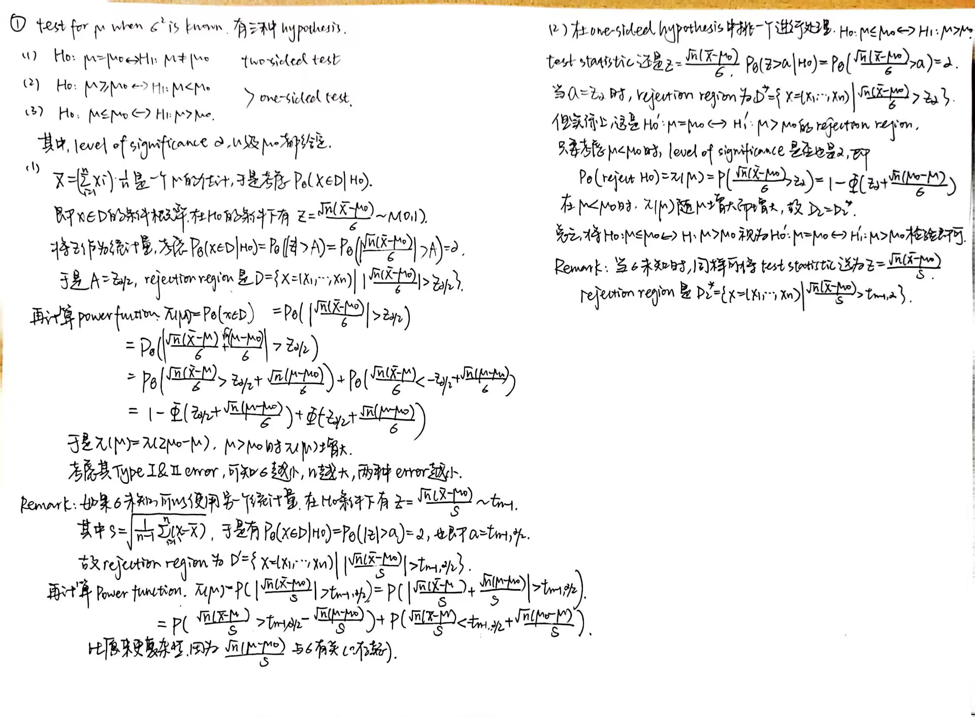
  注意我们在进行检验的时候，往往把等于号的情况归到 null hypothesis 中去。

  以上前半部分对 two-sided 进行了检验，remark 里指出了 \(\sigma\) 未知的检验方法，这称为 \(U\) 检验；后半部分对 one-sided 的一种情况进行了检验，同样在 remark 里指出了 \(\sigma\) 未知的检验方法，这称为 \(t\) 检验。

• 检验 \(\sigma\) 的过程分为是否知道 \(\mu\) 具体值的两种情况，又分为三种典型的 Hypothesis 进行处理，一切都在图中：

  

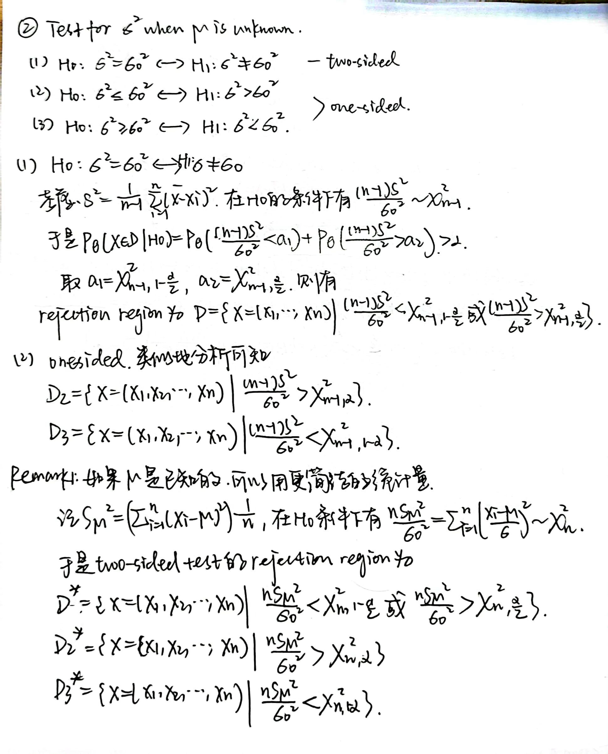
  此处都是利用 \(\chi^2\) 分布进行检验，称为 \(\chi^2\) 检验。

Non-normal population

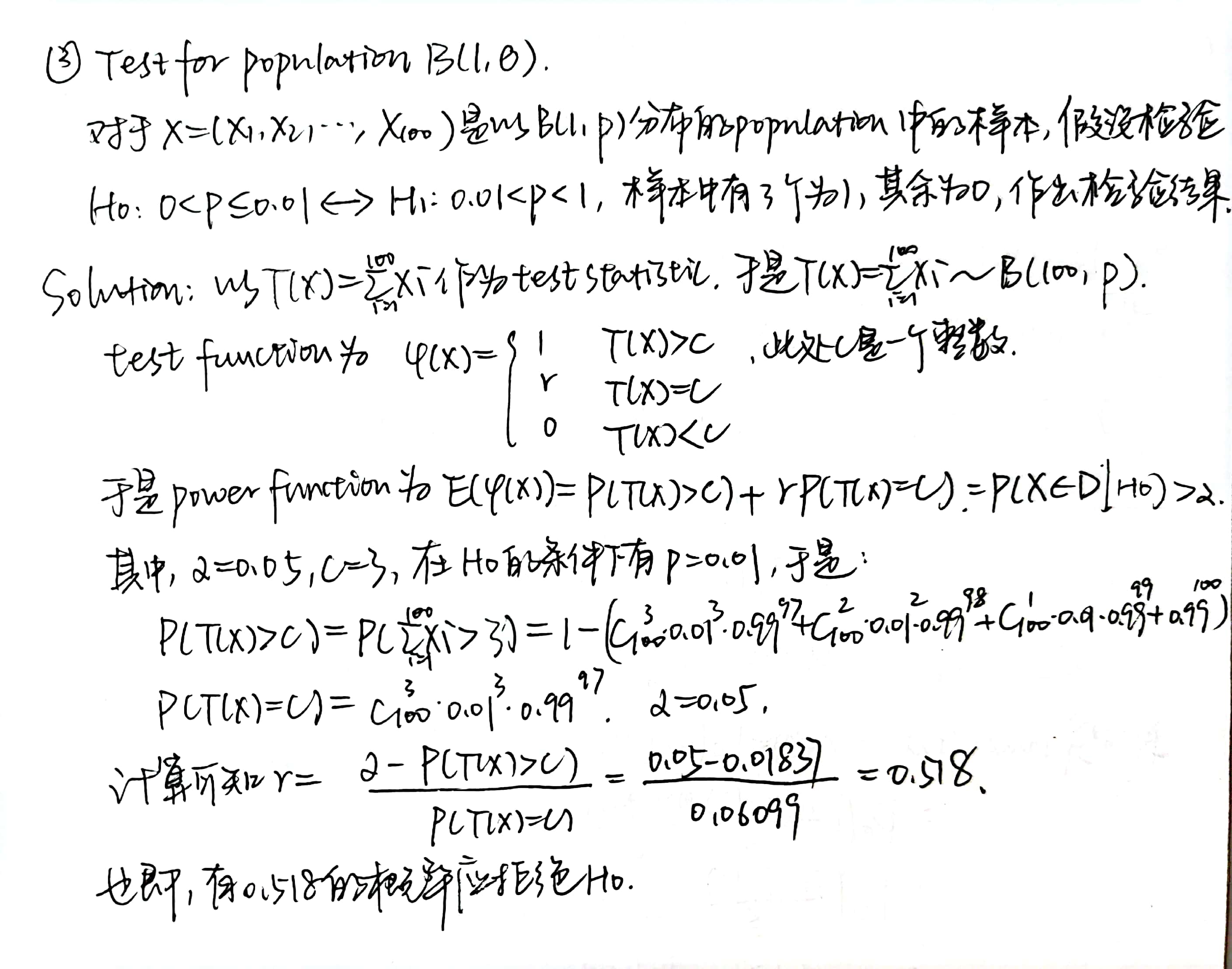
• 检验 \(B(1,\theta)\) 分布的 population 的参数

  以一个例子来说明：

  

  这带我们回顾了 test function \(\varphi(X)\) 的定义，它代表了 \(T(X)\) 取某个值的时候 reject \(H_0\) 的信度。

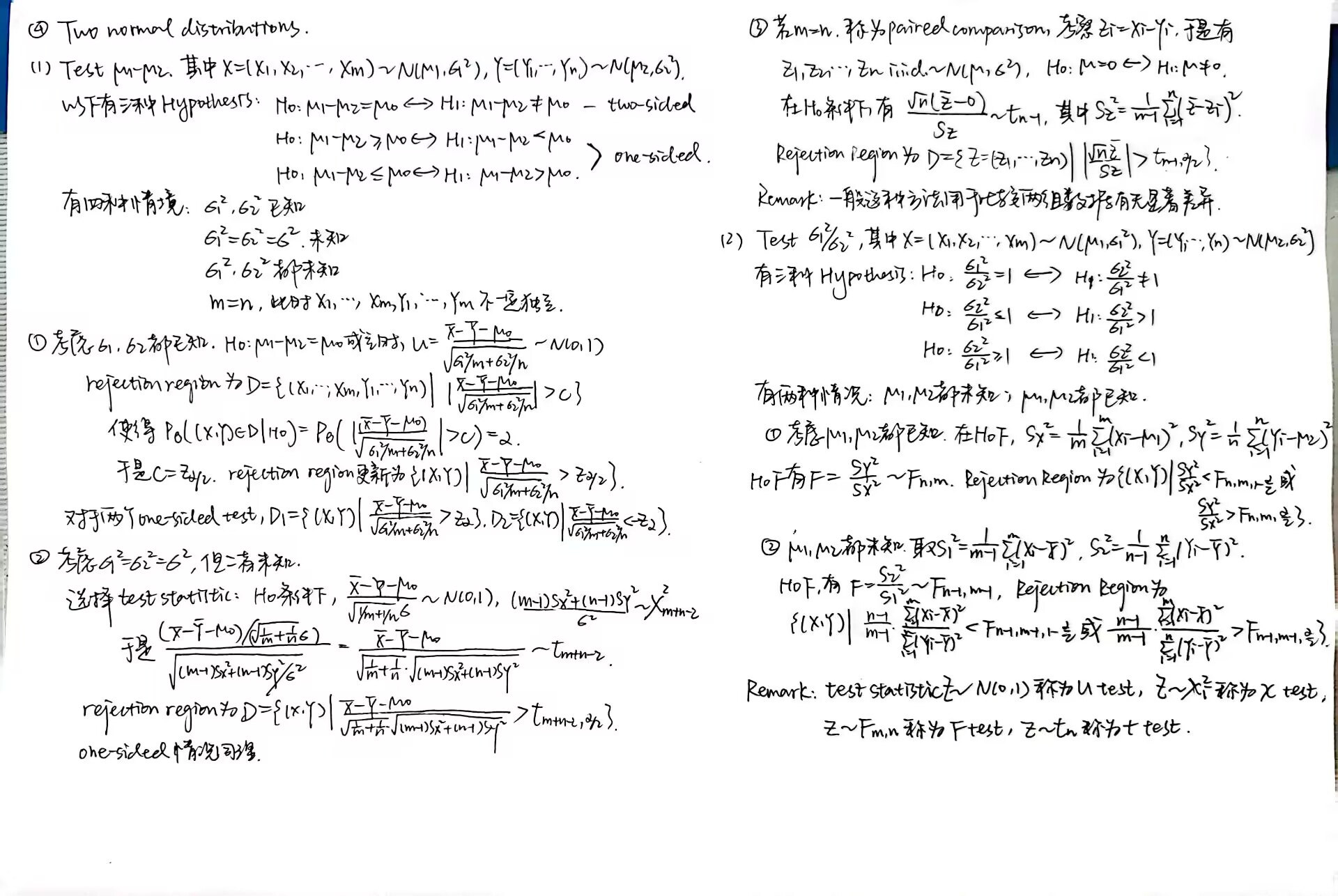
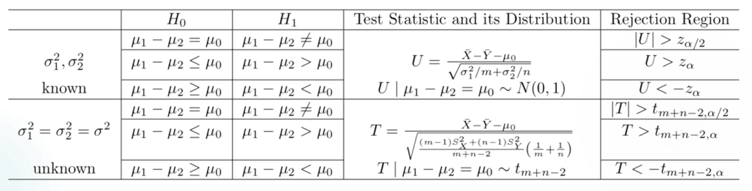
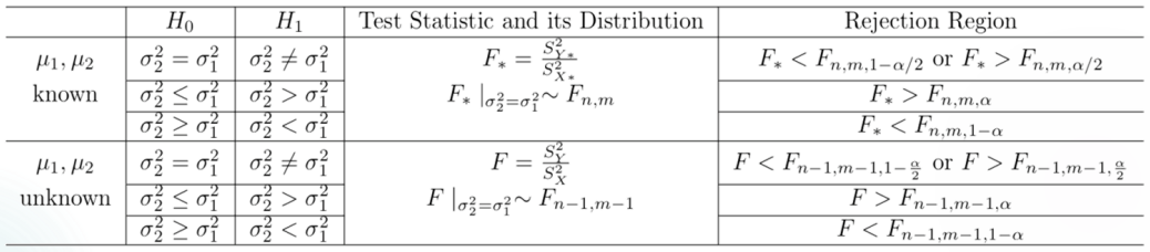
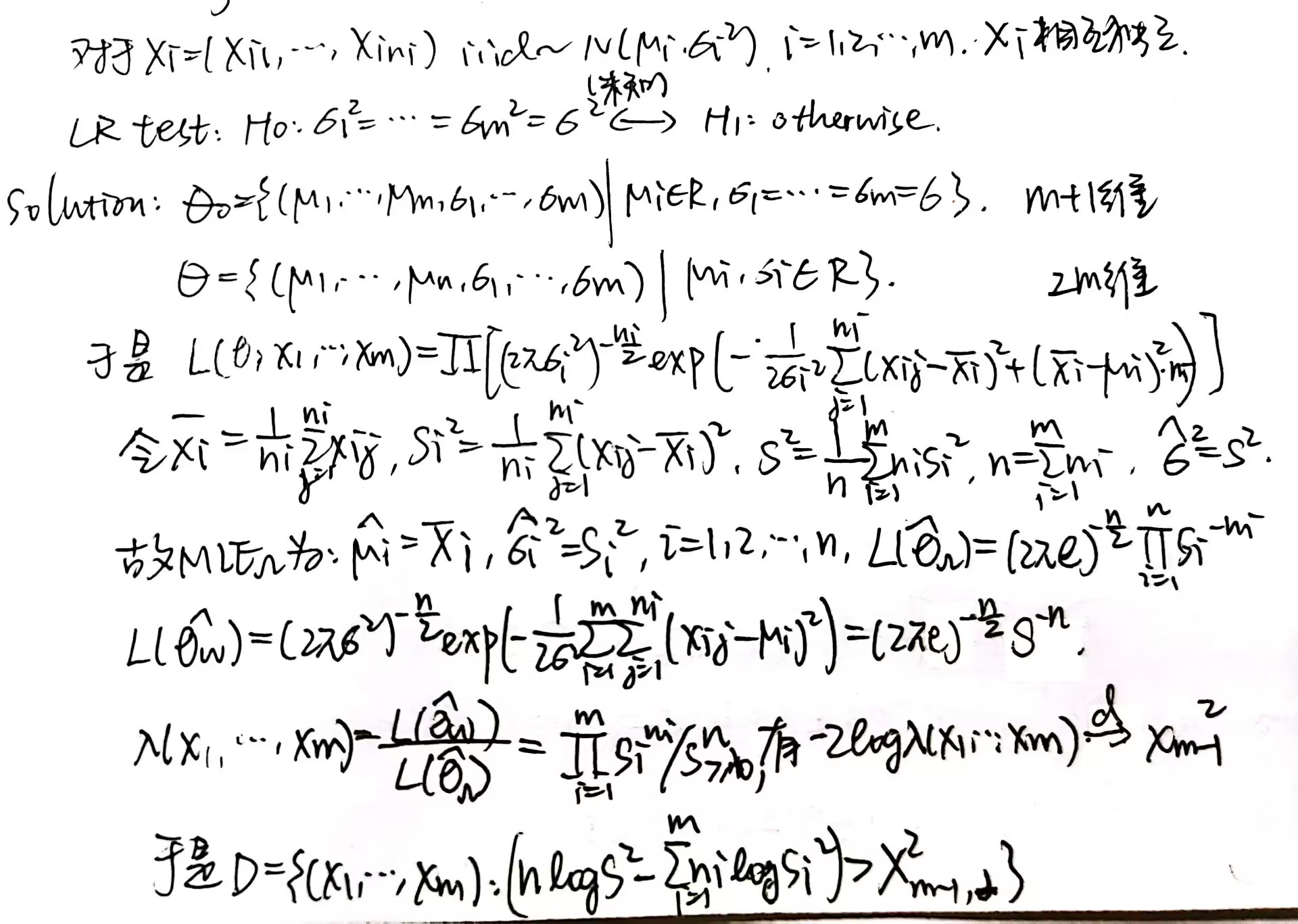
Two normal distributions

• 在 two normal distribution 的情况下，检验 \(\mu_1-\mu_2\)，\(\sigma_1^2 / \sigma_2 ^2\)，以及进行 paired comparison。

  

Summary

本来想自己画个表格，结果摆了。

• One normal population

• Two normal populations（不包括 paired comparison，paired comparison 的目标是考察一个正态分布的期望是否为 0）

• Non-normal population

  \(B(1,\theta)\) 见前。

Bootstrapping Method

本来觉得看起来很好玩，没想到居然直接不讲了，sigh。我自己补一个。

实际情况下样本不一定来自一个 Normal Distribution，数据集也可能不够大。我们可以用 Bootstrap 的方法嗯造一个 Normal Distribution 的数据集，然后进行假设检验。方法是每次有放回地从数据集里抽取一组数据，注意不仅是样本之间可以有重叠，样本内部抽每个数据的时候也是有放回抽取的。

比如对于一个较小的、不确定是否为 Normal Distribution 的数据集做假设检验：\(H_0:\mu = 33.02\)，\(H_1:\mu \neq 33.02\)。

No.	1	2	3	4	5	6	7	8	9	10
Data	28	-44	29	30	26	27	22	23	33	16
No.	11	12	13	14	15	16	17	18	19	20
Data	29	24	24	40	21	31	34	-2	25	19

Bootstrap Method 代码实现如下：

# To see whether datas are from a normal population
speed <- c(28, -44, 29, 30, 26, 27, 22, 23, 33, 16, 24, 29, 24, 40, 21, 31, 34, -2, 25, 19)
hist(speed)

# Create a new population whose mean is 33.02
newspeed <- speed - mean(speed) + 33.02
mean(newspeed)

# Bootstrap Method : Take out 20 observations at random, do it for 1000 times
bstrap <- c()
for (i in 1:1000){
    newsample <- sample(newspeed, 20, replace = T)
    bstrap <- c(bstrap, mean(newsample))
}
hist(bstrap)

# Calculate the p-value: P(stat < 21.75) + P(stat > 44.29)
(sum(bstrap < 21.75) + sum(bstrap > 44.29))/1000

# The p-value is 0.004, which is less than 0.05. Reject H_0

综上，这一组数据不足以支持 \(H_0\)，我们选择 Reject \(H_0\)。

Test based on CLT

实际情况里不一定发生既不是 Normal Distribution，数据集又很小这么背的事情。如果数据量很大的话，完全可以使用 CLT 方法，进行一个 asymptotic sampling distribution 的规约，然后对近似正态分布进行 Hypothesis Testing。

对于一组 \(X_1,X_2,...,X_n i.i.d. \sim F\)，有 mean \(\mu\) 和 variance \(\sigma^2\)，取 \(\bar{X_n}=\Sigma_{i=1} ^n X_i/n\) 为 sample mean，\(S^2 = \Sigma _{i=1} ^n (X_i-\bar{X})^2 /(n-1)\) 为 sample variance。利用 CLT 可知：

\(F=N(\mu,\sigma^2)\) 时，一定有 \(\sqrt{n}(\bar{X_n}-\mu)/\sigma \sim N(0,1)\)。否则 \(n\) 足够大时，由 CLT 也有 \(\sqrt{n}(\bar{X_n}-\mu)/\sigma \to N(0,1)\)。

\(F=N(\mu,\sigma^2)\) 时，有 \(\sqrt{n}(\bar{X_n}-\mu)/S \sim t_{n-1}\)。否则 \(n\) 足够大时，由 CLT 和 Slutsky Theorem，有 \(\sqrt{n}(\bar{X_n}-\mu)/S \to N(0,1)\)。这个形式是用在 \(\sigma\) 未知的场合下进行假设检验的。

以上二者均依分布收敛。

• Test \(\mu_1 -\mu_2\) when \(\sigma_1 ^2,\sigma_2 ^2\) unknown, and m, n are both large enough

  由 CLT 和 Slutsky Theorem，可知在 \(H_0:\mu_1 -\mu_2 =\mu_0\) 条件下，\(U=\frac{\bar{Y}-\bar{X}-\mu_0}{\sqrt{S_X ^2 /m+ S_Y ^2 /n}} \to N(0,1)\)。对其假设检验，得到双尾检验的 Rejection Region 是 \(D=\lbrace (X_1,...,X_m,Y_1,...,Y_n) | |U|>z_{\alpha /2} \rbrace\)。

• Test the mean \(\theta\) of \(B(1,\theta)\) when n is large enough

  由 CLT 可知在 \(H_0:\theta = \theta_0\) 条件下，\(U=\frac{\sqrt{n}(\bar{X}-\theta_0)}{\sqrt{\theta_0(1-\theta_0)}} \to N(0,1)\)，双尾检验的 Rejection Region 为 \(D=\lbrace (X_1,...,X_n) | |U| > z_{\alpha /2} \rbrace\)。

• Test the mean \(\theta\) of \(P(\theta)\) when n is large enough

  由 CLT 可知在 \(H_0:\theta = \theta_0\) 条件下，\(U =\frac{\sqrt{n}(\bar{X}-\theta_0)}{\sqrt{\theta_0}} \to N(0,1)\)，双尾检验的 Rejection Region 为 \(D=\lbrace (X_1,...,X_n) | |U| > z_{\alpha /2} \rbrace\)。

Homework 5

略麻烦，我不是很懂那个 \(B(1,\theta)\) 的自主检验方法，蹲一个标答。

Lecture 10

老师发着烧还坚持上课，辛苦了 qwq

本节继续介绍 Hypothesis Testing，但是使用 Likelihood Ratio 方法。

Likelihood Ratio Test (LRT)

我们之前知道，解 MLE 方法的原理是 Likelihood Function 的值越大，说明 \(\theta\) 作为参数的可能性越大。在 Hypothesis Test 中也可以通过 \(H_0,H_1\) 的 maximum likelihood 得到最佳的 \(\theta\)，从而对 \(H_0,H_1\) 做判断。

为了方便后续的计算，我们先给出：对于一个 random sample \(X_1,...,X_n i.i.d. \sim N(\mu,\sigma ^2)\)，在 MLE 那一讲已经求得，其 \(\hat{\mu}_{MLE} = \bar{X}\) 是 sample mean，但 \(\hat { \sigma } _{MLE} ^2\) 不是 sample variance，而是 \(\frac {1} {n} \Sigma _{ i=1 } ^n (x _i - \mu) ^2\)。

Likelihood Ratio Method

• \(H_0:\theta =\theta_0 \leftrightarrow H_1:\theta =\theta_1\)，一个不是非常寻常的 hypothesis test。

  考虑 \(\frac{L(\theta_0; x)}{L(\theta_1; x)} <c\) 时 reject \(H_0\)。显然，如果 accept \(H_1\)，则说明全域 \(\Theta\) 上的最佳参数是 \(\theta_1\)，也即它是 MLE，使得 \(L(\theta_1;x)>L(\theta_0;x)\) 成立。于是在 hypothesis test 中放松些要求，考虑 \(\frac{L(\theta_0; x)}{L(\theta_1; x)} <c\) 时 Reject \(H_0\)。

• 推广到 \(H_0:\theta \in \Theta_0 \leftrightarrow H_1:\theta \in \Theta_1\)

  考虑 \(\frac{sup_{\theta \in \Theta_0} L(\theta;x)}{sup_{\theta \in \Theta_1} L(\theta;x)} <c\) 时 reject \(H_0\)。这个想法也很自然，\(sup_{\theta \in \Theta} L(\theta;x)\) 对应的 \(\theta\) 就是 \(\Theta\) 域中最佳的参数取值。

  实际上，我们可以把 \(sup _{\theta \in \Theta _0 } L(\theta ; x )\) 记作 \(L( \hat { \theta } _{MLE ; 0} )\)。

  同样地，把 \(sup _{\theta \in \Theta } L(\theta;x)\) 记作 $ L( _{MLE} )$。

  于是当 \(L(\hat{\theta} _{MLE; 0} )\) / $ L( _{MLE} )$ 接近于 \(1\) 时，\(H_0\) 更有可能是对的；如果 \(L(\hat{\theta} _{MLE; 0} )\) / \(L(\hat{\theta} _{MLE} )\) 距离 \(1\) 比较远，就更有可能是错的。

• 记 likelihood ratio 为 \(\lambda (x) = L(\hat{\theta} _{MLE; 0} )\) / \(L(\hat{\theta} _{MLE} )\) ，于是当 \(\lambda(x)<\lambda_0\) 时 reject \(H_0\)，其中 \(\lambda_0\) 是一个等待被决定的常数。

  决定这个常数的过程和上一讲的操作基本上是一样的。一般来说，我们会把 reject \(H_0\) 的条件等价地写成：\(-2 log \lambda > C(=-2log \lambda_0)\)，然后对于 continuous / discrete distribution 进行讨论。

  对于 non-randomized test，\(\varphi (x) = I_{\lbrace \lambda < \lambda_0 \rbrace}\)，考虑 \(\pi(x) = E_\theta \varphi(X) \leq \alpha\)。

  对于 randomized test，在 \(\lambda=\lambda_0\) 处插入 \(\varphi(x)=r\)，\(r\) 是一个 \((0,1)\) 上的值即可。

单 Population 上样本的 LRT

单 Normal Distribution 上样本的 LRT

双 Normal Distribution 上样本的 LRT

饶了我罢。

PPT 第 27-36 页，自行查阅，此处略过。

Limiting Distribution of LR

• 如果 \(\Theta\) 的维度为 \(k\) 严格大于 \(\Theta_0\) 的维度 \(s\)，分布的 PDF 符合正则条件，则对于检验问题 \(H_o:\theta \in \Theta_0 \leftrightarrow H_1 : \theta \in \Theta_1\)，在 \(H_0\) 条件下，当 \(n \to \infty\) 时有 \(-2log \lambda(X) \to \chi _t ^2\) 依分布收敛，\(t=n-s\)。

• Example 1：

  

• 总的来说，对于一个大样本，我们对 \(H_0:\theta \in \Omega_0 \leftrightarrow H_1:\theta \notin \Omega_0\) 进行 LRT 时，LR 即为 \(\lambda=\frac{max_{\theta \in \Omega_0} L(\theta)}{max_{\theta \in \Omega} L(\theta)}\) 且使得 \(-2log\lambda \to \chi_t ^2\)。于是 reject \(H_0\) 的条件即为 \(-2log \lambda>-2log \lambda_0=\chi_{t,\alpha} ^2\)，由此可以确定 \(\lambda_0\)。

• Application: (Hardy-Weinberg equilibrium) 一个基因可以表达为 \(A\) 或者 \(a\)，组合成为 \(AA,Aa,aa\) 之一。对于观察到的基因样本，我们已知一个样本量为 \(n\) 的样本中每种基因的个数，记为 \(N_{AA},N_{Aa},N_{aa}\)。希望通过这一数据，推算出基因表达为 \(A\) 的概率 \(\theta\)。（以我高一上学期生物期中考试 42 分的水平勉强表达完了题面，真不懂这个东西）考虑如下：

  • Hardy-Weinberg equilibrium 的 null hypothesis 为：\(H_0: p_{AA}=\theta^2\)，\(p_{Aa}=2\theta (1-\theta)\)，\(p_{aa}=(1-\theta)^2\) 对某个 \(\theta \in (0,1)\) 成立。对应的 alternative hypothesis 即为 otherwise。用 LRT 进行检验：

  • \(\Theta_0=\lbrace (p_{AA},p_{Aa},p_{aa} )| p_{AA}=\theta^2\)，\(p_{Aa}=2\theta (1-\theta)\)，\(p_{aa}=(1-\theta)^2 \rbrace\) 是一维的，因为变量实际上只有 \(\theta\)。

    \(\Theta=\lbrace (p_{AA},p_{Aa},p_{aa} )| p_{AA}+p_{Aa}+p_{aa}=1\rbrace\) 是二维的，因为它由一个线性式决定。故 \(t=n-s=1\)。

  • 于是 $ =( { {AA} })^{N {AA} }$ \(( \frac{ \hat{p} _{0,Aa} } {\hat{p} _{Aa} }) ^{N _{Aa} }\) \((\frac{\hat{p} _{0,aa} } {\hat{p} _{aa} } ) ^{N _{aa} }\)。

  • Full-model MLE 是 \(\hat{p} _{AA}=N _{AA} /n\)，\(\hat{p} _{Aa}=N _{Aa}/n\)，\(\hat{p} _{aa}=N _{aa}/n\)。

  • 而 sub-model 的 MLE 可以计算 Likelihood Function 得到，为 \(\hat{\theta} = \frac{2N_{AA}+N_{Aa}}{2n}\)。

    对应可求得 \(\hat{p} _{0,AA}\)，\(\hat{p} _{0,Aa}\)，\(\hat{p} _{0,aa}\)，再代入 \(-2log\lambda \to \chi_1 ^2\) 就可以求出 rejection region，是一个 \(\chi^2\) 检验的形式。

Summary

没想到今天又熬了个通宵学统推，很酣畅淋漓的感觉。问就是生活在东四区。

沃日，修炸掉的 LaTeX 又修了半个小时， 这下快到东三区了。

LRT 的内容其实说白了和费尽心思找 test statistic 的 Hypothesis Test 求法没有区别，最后困难的点还是收敛到了找参数上面。LRT 是借助 level of significance 以及视 \(\lambda(x)\) 为 rejection region 的雏形来找 \(\lambda_0\)，上一讲的检验找的是分位数，差不多的事。

Lecture 11

Hypothesis Test 的最后一讲，关于 Universal Most Powerful Test，理解起来真的很折磨王。

UMP Test

• Definition：对于某些特定的 hypothesis：\(H_0: \theta \in \Theta_0 \leftrightarrow H_1 : \theta \in \Theta_1\)，如果 power function 在 \(\Theta_0\) 上的取值满足 \(\beta _{\varphi} (\theta)=E _\theta [\varphi (X)] \leq \alpha, \forall \theta \in \Theta_0\)，则记 test function \(\varphi(x)\) 是一个 level \(\alpha\) test。

  此时，记 \(\Phi _{\alpha} = \lbrace \forall \varphi (x): \beta _{\varphi} (\theta) \leq \alpha , \theta \in \Theta_0 \rbrace\) 是一系列满足 power function 的检验，如果其中存在某个检验 \(\varphi ^* (x) \in \Phi _{\alpha}\) 使得对任意的 \(\varphi (x)\)，有 power function 在 \(\Theta_1\) 上的任意取值也满足 \(\beta _{\varphi ^*} (\theta) \geq \beta _{\varphi } (\theta)\)，那么称检验 \(\varphi ^* (x)\) 是一个 uniformly most powerful level \(\alpha\) test。

  说人话：对于一些 Type I Error 发生概率不超过 \(\alpha\) 的检验，其中 Type II Error 也最小（也就是说 \(\beta(\theta)\) 在 \(\theta \in \Theta_1\) 上取值总是最大）的那个就是 UMP test。

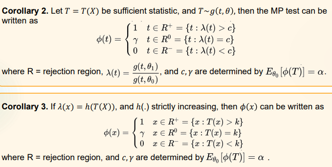
• Neyman-Pearson Lemma 是一个在双单假设检验中寻找 UMP test 的充要条件。定理叙述为：

  对于 Hypothesis \(H_0: \theta = \theta_0 \leftrightarrow H_1 : \theta = \theta _1\)，分布对应 PDF 或 PMF 为 \(f(x | \theta_i)\)，有某个 test 满足以下条件：

  • 如果 \(\frac{f(x|\theta _1)}{f(x|\theta _2)} > k\)，则有 \(x \in D\)，样本在 \(H_0\) 的 rejection region 中。
  • 如果 \(\frac{f(x|\theta _1)}{f(x|\theta _2)} < k\)，则有 \(x \in D^c\)，样本不在 \(H_0\) 的 rejection region 中。
  • \(\alpha = P _{\theta _0} (X \in D | H_0)\)，即 Type I Error 发生的概率是 \(\alpha\)。

  其中 \(k\) 是某个非负数，\(\alpha\) 是设定好的 level of significance。

  于是这个 test 是 UMP level \(\alpha\) test。反过来对于一个 UMP test，也一定满足上述条件，也就是说按照 Likelihood Ratio 的范围来确定 rejection region。

• Neyman-Pearson Fundamental Lemma 是一个关于 discrete distribution 的更详细叙述。

  对于 Hypothesis \(H_0: \theta = \theta_0 \leftrightarrow H_1 : \theta = \theta _1\)，分布对应 PMF 为 \(f(x | \theta_i)\)，样本为 \(X=(X_1,...,X_n)\)，于是 test function 记为：\(\varphi(x)\) 在 \(\frac{f(x|\theta _1)}{f(x|\theta _2)} > k\) 时取 \(1\)，在 \(\frac{f(x|\theta _1)}{f(x|\theta _2)} < k\) 时取 \(0\)，在 \(\frac{f(x|\theta _1)}{f(x|\theta _2)} = k\) 时取 \(r\)。

  于是存在 \(k>0,0<r<1\) ，使得 \(E _{\theta _0} \varphi(X)= P _{\theta _0} [\frac{f(x|\theta _1)}{f(x|\theta _2)} > k] + r P _{\theta _0} [\frac{f(x|\theta _1)}{f(x|\theta _2)} = k] = \alpha\) ，这个 test 是所有 level of significance 小于 \(\alpha\) 的 test 的 UMP。注意上式是一个在 \(H_0\) 下的条件概率，表征 Type I Error 的概率。在具体例子里，我们可以通过这个式子确定 \(r\) 的取值。

  当然，如果是 continuous distribution，\(r=0\)，同样做检验即可。

• Corollary：有三条推论，但是懒得写了。

  • 对某个 Hypothesis 的 UMP level \(\alpha\) test，它的 power function 在 \(\Theta_0\) 上取值是 \(\alpha\)，所以在 \(\Theta_1\) 上大于等于 \(\alpha\)。

  • 关于充分统计量的两条。感觉不太会拿来考试就直接截个屏吧。证明也不难。

    

• Applications：

  • Example 1：

    

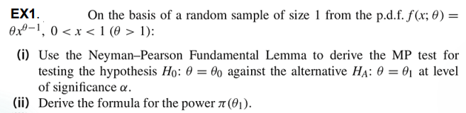
    Discussions for Example 1：

    

    

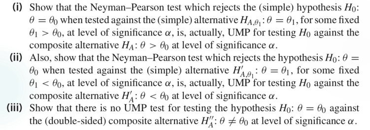
    Remark：这个很典型，从单点推广到单侧检验，但是双侧检验是行不通的。

  • Example 2：

    

    

    Remark：因为会做所以就不手写了，截个图当存档。可以当做 UMP 系列中 randomized test 的范本。

  • Example 3：

    

    

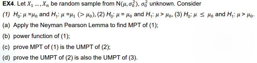
    Remark：最后一问下次再看看。

UMP Test 问题的常见规约

在上面的 Application Examples 里面我们看到，UMP Test 问题有很多规约情况，可以通过两个单点 hypothesis 先归到一个单点，再推广到双区间情况。也有时候双侧检验不能规约。下面对于一般的情况进行讨论。

• \(\varphi (x)\) 是 hypothesis \(H_0 : \theta = \theta _0 \leftrightarrow H_1 : \theta = \theta _1 (\theta _1 > \theta _0)\) 的一个 \(\alpha\) level 检验。如果 \(\varphi(x)\) 的取值不依靠 \(\theta _1\) 而存在，则上述 hypothesis 可以推广到 \(H_0 : \theta = \theta _0 \leftrightarrow H_1 : \theta > \theta _0\) 形式。

• Example 1：

  

  

  Remark：第二问里面是一个双侧检验，但是 rejection region 仍然是单侧的。说明二者之间没有必然的关系。

• Example 2：

  

  

• Summary：做一般复合假设的 MP 的步骤，general hypothesis 记为 \(H_0: \theta \in \Theta _0 \leftrightarrow H_1: \theta \in \Theta _1\)。

  • 在 \(\Theta _0\) 里寻找一个尽量靠近 \(\Theta _1\) 的点 \(\theta _0\)，在 \(\Theta _1\) 里同样找一个 \(\theta _1\)。
  • 按照 NP lemma 来建立一个关于 \(H_0: \theta = \theta _0 \leftrightarrow H_1: \theta =\theta _1\) 的 MP，记为 \(\varphi _{\theta _1}\)。
  • 如果 \(\varphi _{\theta _1}\) 关于 \(\theta _1\) 独立，则它可以扩充到 \(H_0: \theta =\theta _0 \leftrightarrow H_1: \theta \in \Theta _1\) 的 UMP。
  • 想要再扩充到 \(H_0: \theta \in \Theta _0 \leftrightarrow H_1: \theta \in \Theta _1\) 的话，需要检验 power function 在 \(\Theta_0\) 里的取值，也即验证 \(E _\theta \varphi (X) \leq \alpha,\theta \in \Theta_0\)。一般来说，如果 power function 是单调的，这个条件比较容易满足，而这在单参数指数分布族中比较常见。
  • 以上方法对单维度参数可行，且要求参数空间在 \(R\) 上。分布属于单参数指数分布族。

• Fun Fact：实际上是先有了 N-P Lemma，人们才回头构造了 Likelihood Ratio Test，最后才有最开始学习的 F-test，t-test 之类的东西。

Hypothesis Testing & Confidence Interval

之前做题的时候一直感觉到这二者之间有关系，下面用定理和一个简单的一菜两吃（x）的例子详细说一下为什么其实是一回事，也作为 hypothesis testing 学习的尾声。

• Example：

  

  

• Summary：实际上我们再看这个过程。以寻找 CI 为例。

  • 把目标转化为 Test the hypothesis： \(H_0: \theta = \theta _0 \leftrightarrow H_1: \theta \neq \theta _0\)，要求 level of significance 为 \(\alpha\)。然后来计算 \(\theta\) 的 confidence interval \([\hat{\theta} _1 (X),\hat{\theta} _2 (X)]\)，有 confidence level 为 \(1-\alpha\)。

  • 在 \(H_0\) 条件下，如果 \(\theta \notin [\hat{\theta} _1 (X),\hat{\theta} _2 (X)]\)，我们就 reject \(H_0\)。这一概率是 Type I Error 概率：

    \(P(reject | H_0)=P_{\theta _0}(\theta _0 \notin [\hat{ \theta } _1 (X), \hat { \theta } _2 (X) ]) = 1 - P _{ \theta _0} ( \theta _0 \in [\hat{ \theta} _1 (X),\hat{ \theta} _2 (X)]) = \alpha\)

  • 所以 \([\hat{\theta} _1 (X),\hat{\theta} _2 (X)]\) 是一个以 confidence level \(1-\alpha\) 的 confidence interval

  寻找 upper confidence limit 则检验 hypothesis：\(H_0: \theta \geq \theta _0 \leftrightarrow H_1: \theta < \theta _0\)；

  寻找 lower confidence limit 则检验 hypothesis：\(H_0: \theta \leq \theta _0 \leftrightarrow H_1: \theta > \theta _0\)。

• Theorem 1：对任意的 \(\theta \in \Theta\)，有一个 hypothesis \(H_o:\theta = \theta _0\) 的检验，它的 level of significance 是 \(\alpha\)，而 \(H_0\) 的 acceptance region 是 \(A(\theta _0)\)。于是集合 \(C(X)= \lbrace \theta : X \in A(\theta) \rbrace\) 是一个以 \(1-\alpha\) 为 confidence level 的 confidence region for \(\theta\)。

• Theorem 2：\(C(X)\) 是一个以 \(1-\alpha\) 为 confidence level 的 confidence region for \(\theta\)，也就是对任意 \(\theta _0 \in C(X)\)，有 \(P[\theta _0 \in C(X) | \theta = \theta _0] = 1- \alpha\)。于是 hypothesis \(H_0 : \theta = \theta _0\) 的 acceptance region 是 \(A(\theta _0)=\lbrace X : \theta _0 \in C(X) \rbrace\)，这一 test 的 level of significance 是 \(\alpha\)。

Extended Content *

总之就是好玩的东西。

Monotone Likelihood Ratio

对于某个 sample 的充分统计量 \(T(X)\)，考虑关于它的检验使得以 \(T(x)\) 为 rejection region 的度量。

UMP in Exponential Family

• \(X_1,X_2,...,X_n\) 是一组来自 exponential family 的 random sample，它们的 population 服从一个以 $f(x;) = C() h(x) exp(Q() T(x)) $ 为 PDF 的 distribution。其中，\(Q(\theta)\) 是严格单调的。由 exponential family 的性质，我们记 \(V(x_1,...,x_n) = \Sigma _{i=1} ^n T(x_i)\) 为一个 sufficient statistic。

  如果 \(Q(\theta)\) 严格递增，考虑 hypothesis \(H_0: \theta \leq \theta _0 \leftrightarrow H_A : \theta > \theta _0\)，UMP test 的形式由 test function 给出： \(V(x_1,...,x_n)>C\) 时 \(\varphi (x_1,...,x_n) = 1\)，\(V(x_1,...,x_n)<C\) 时 \(\varphi (x_1,...,x_n) = 0\)， \(V(x_1,...,x_n) = C\) 时 \(\varphi (x_1,...,x_n) = \gamma\)。根据 level of significance 是 \(\alpha\)，可以确定出 \(\gamma\) 的取值。

  hypothesis 的形式为 \(H_0: \theta \geq \theta _0 \leftrightarrow H_A : \theta < \theta _0\) 的做法类似，\(Q(\theta)\) 单调递减时的操作也类似。

• 可以这么做的原因是，这和使用 likelihood function 的结果是一样的。

  先考虑单点 hypothesis \(H_0: \theta = \theta _0 \leftrightarrow H_A : \theta = \theta _1(\theta _1 > \theta _0)\)，此时有 \(\lambda (x)=\frac{f(x; \theta _1)} {f(x; \theta _0)}\) 是关于 \(V(x)\) 严格单调的，由此可以给出单点处的 MP Test，它不依赖于 \(\theta _1\)，可以把 \(H _A\) 延拓到 \(\theta > \theta _0\)。而 power function 在 \(\Theta _0\) 上是关于 \(\theta\) 单调的，可以再把 \(H_0\) 延拓到 \(\theta \leq \theta _0\)。

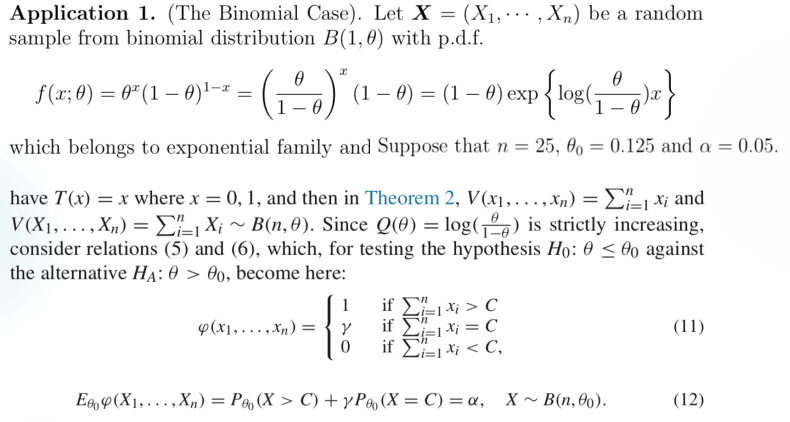
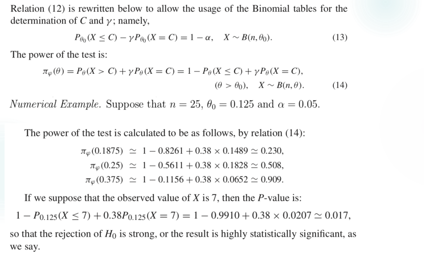
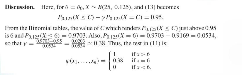
• Example 1：The Binomial Case

  

  

  

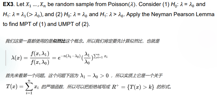
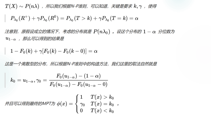
Homework 6

破事挺多啊

助教在干啥助教为什么不批作业了（

Lecture 12

最后一课，介绍一些分布未知时的处理方法，称为非参数检验。

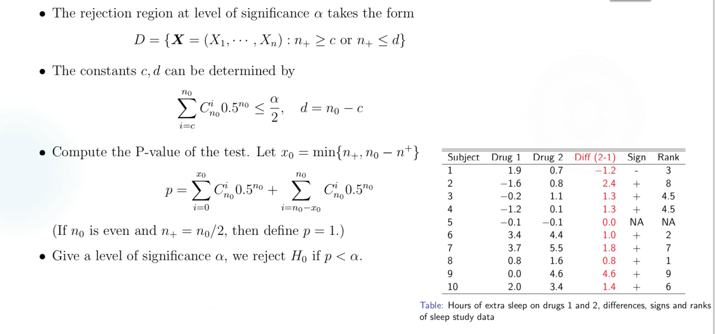
Sign Test

• 对于 paired data 的检验。

  假定 \(X=(X_1,...,X_n),Y=(Y_1,...,Y_n)\) 是已知的两组数据，希望知道二者之间有没有显著差异，即 hypothesis 为 \(H_0: \mu = 0 \leftrightarrow H_1 : \mu \neq 0\)，其中记 \(Z_i = Y_i - X_i,\mu = E(Z_i)\)。

  实际上我们也可以通过 two sample t test 进行操作，假设 \(X,Y\) 是正态分布的。但是这样做精度不高，而且无法突出两组数据的特征，尤其是在有明显偏离的数据上，non-parametric test 表现更好。

  说回主题，在 sign test 中我们可以赋予每一个 data 一个 sign 值，以祈这一组 sign 值近似于某一分布。最简单的方式就是按照 data 的正负性来赋值，记 \(n_+\) 为 sign 的正值数量，\(n_-\) 为负值数量，舍弃 \(0\) 值。于是有 \(n_0 = n_+ + n _-\)，且 \(n_+ \sim B( n_0 , \theta)\)，原假设即转化为 \(H_0 : \theta = 0.5 \leftrightarrow H_1 : \theta \neq 0.5\)，变成了熟悉的检验形式。

• Example for paired test

  

  

• Test median of population

  通过一个样本来找某一 population 的中位数，也可以通过 sign test 进行，放一个例子在这里，就不细说了。

  

  

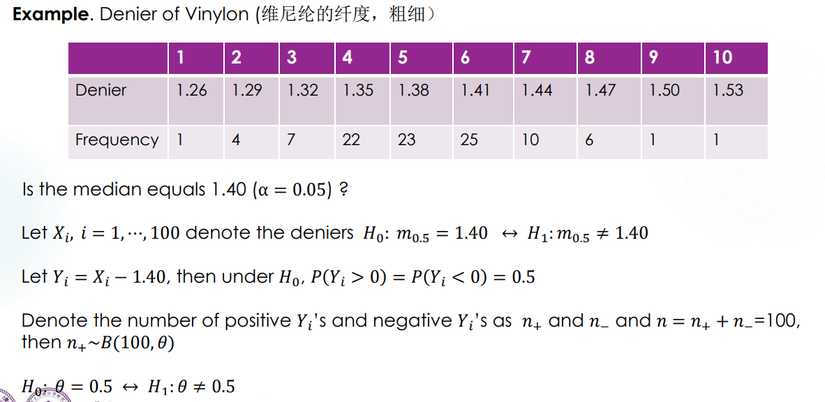
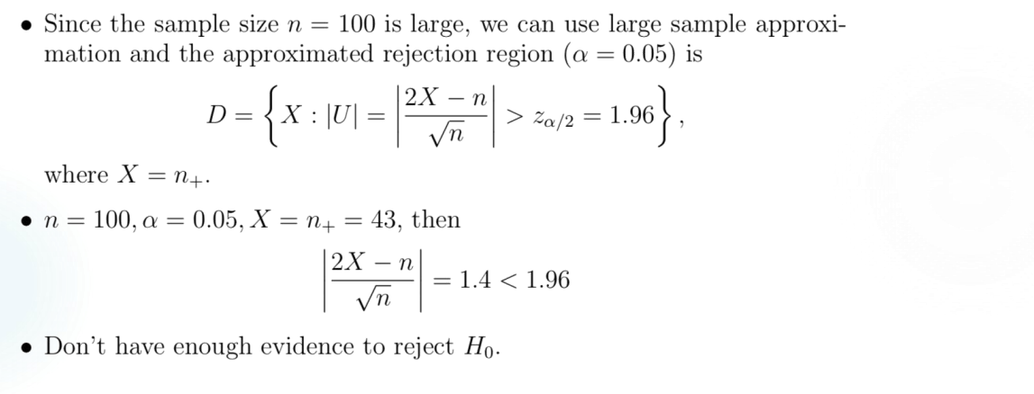
  Remark：实际上在这个例子里，取 median 为 1.39 也不影响检验结果。sign test 对具体数据的表现能力较弱，实际上是 low power 的。

Wilcoxon Signed Rank Sum Test

这个东西很好玩，但是考试暂时不考，码的成分又比较大，而且理论部分我想后面再研究研究再写，先跳过了。

Goodness of Fit Test

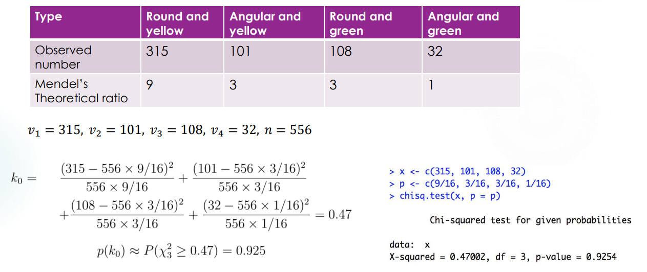
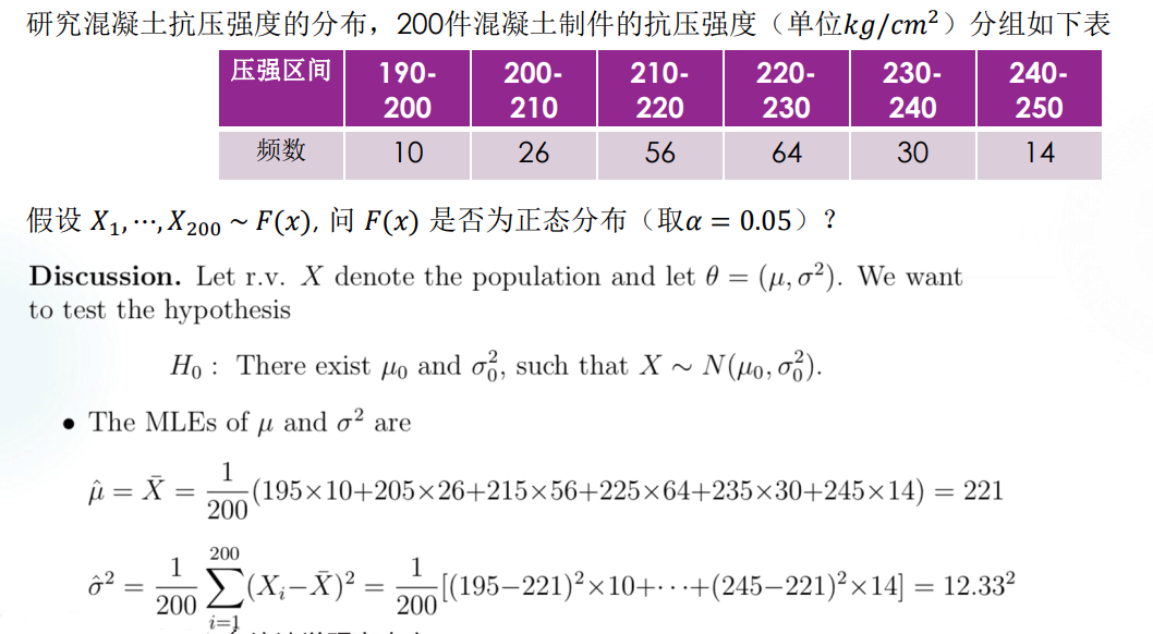
难得遇到一个我早就考虑过的问题，大概是高一上生物课的时候，讲孟德尔种豌豆发现某些基因表达的比例大概是 \(9:3:3:1\)。我就很好奇这个是怎么近似出来的，你总不能只告诉我“看着很像”吧。Goodness of fit test 大概就是解决这一类问题。

• 设 \(X=(X_1,...,X_n)\) 是来自某一 population 的随机样本，\(F\) 是一个给定的分布，也叫做 theoretical distribution，我们想要验证 \(H_o: X \sim F\) 这一假设。

  首先我们需要进行一些量化，来反映某个 statistic 什么情况下能代表 \(X \sim F\)。也就是说，要定义一个 quantity \(D=D(X_1,X_2,...,X_n,F)\) 使得在 \(D \geq c\) 时 reject \(H_0\)。这时定义 goodness-of-fit 的程度为 \(p(d_0) = P(D \geq d_0 | H_0)\)，\(d_0\) 是确切样本下 \(D\) 的观测值。

• Pearson \(\chi ^2\) test for discrete F

  令 \(X=(X_1,X_2,...,X_n)\) 是 population \(X\) 中的一个随机样本，theoretical distribution \(F\) 为一个离散分布，其 PMF 为 \(f(a_i)=p_i,\Sigma _{i=1} ^r p_i =1\)。于是 hypothesis 转化为 \(H_0: P(X=a_i) = p_i,i=1,2,...,r\)。

  记 \(v_i\) 是样本中观察到的 \(a_i\) 的出现次数，于是 \(\Sigma _{i=1} ^r v_i= n\)，\(v_i\) 是自然数。在 \(H_0\) 条件下，当 \(n\) 足够大时，有频率 \(\frac { v_i }{n} \to p_i\)。于是我们用 \(K_n = \Sigma _{i =1} ^r c_i (\frac {v_i}{n} -p_i) = \Sigma _{i=1} ^r \frac{(v_i - np_i) ^2}{np_i }\) 作为衡量的指标，其中的系数 \(c_i = \frac{n} {p_i }\)。

  这一指标的好处在于，在 \(H_0\) 条件下，当 $n $ 时有 \(K_n \to \Chi _{r-1} ^2\)。所以称为 Pearson \(\chi ^2\) test。

• Example 1：

  

• Pearson \(\chi ^2\) test for continuous F

  这和数值分析里面那个差分技巧还挺像的，分割区间然后强行转成 discrete distribution 就可以了。取 \(r-1\) 个常数 \(a_0 = -\infty < a_1 < a _2 <...< a _{r-1} < + \infty = a _r\)，就把区间分割成了 \(r\) 段（注意它们的起和止，除了 \(I_r\) 之外都是左开右闭的）：\(I _1 = (- \infty , a _1], I_2 = (a_1, a_2],..., I _r = (a _{r-1} , \infty)\)。再记 \(p_j = P _F(X \in I_j) = F(a_j) - F(a _{j-1})\) 即可做出假设：\(H_0 : P(X \in I_j) = p_j,j=1,2,...,r\)。

  类似地给出衡量指标 \(K_n = \Sigma _{i =1} ^r c_i (\frac {v_i}{n} -p_i) = \Sigma _{i=1} ^r \frac{(v_i - np_i) ^2}{np_i }\)，在 \(H_0\) 条件下，当 $n $ 时有 \(K_n \to \Chi _{r-1} ^2\)。

  Remark：可以看到这个操作的近似程度做得比较多，所以有几点注意事项。

  • 关于 \(r\) 的选择。理论上和实际观测到的 frequency \(v_i\) 不能小于 \(5\)，否则应当合并相邻的区间。
  • 不能根据得到的 sample 来划定 \(a_i\)，这是没有普遍性的。
  • 实际上因为左右端是取到无穷的，这一区间的选择方式可能带来一定问题。

• Example 1：

  

  

  

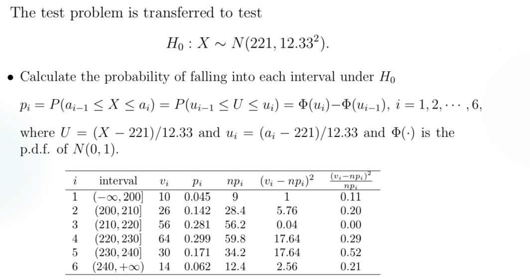
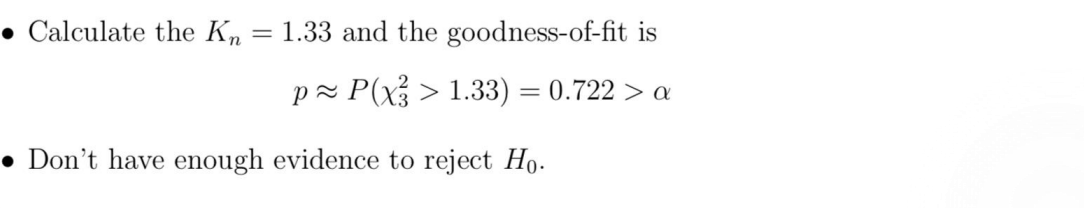
  Remark：可以看到这里 Pearson 指标的近似分布是 \(\chi ^2 _3\) 而不是 \(\chi ^2 _5\)，这是因为此处的 theoretical distribution 参数也是未知的，是通过 MLE 方法估计出来的。在这种情况下，Pearson 指标将收敛到 \(\chi ^2 _{r-s-1}\)，其中 \(s\) 是未知参数的数目。

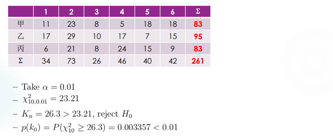
Contingency Table Independence

另一种问题，种豌豆的时候每一次收获的结果必然有数值上的差异，（开始认真地编数据），比如说第一次是 \(213 : 76 : 69 : 25\)，第二次是 \(254 : 85 : 89 : 32\)，那么凭什么说它们都反映了同样的比例？

我们称 \(10\) 次采集豌豆统计出来的表格为 contingency table，contingency 为偶然的意思，称这种检验为 homogeneity test，即为同质性检验。（词汇量 ++！（

• 实际上，我们用一个高维的 \(\chi ^2\) 检验来解决问题。Contingency table 的形式如下：

  	Category 1	...	Category C	\(\Sigma\)
  Group 1	\(N_{11}\)	...	\(N_{1C}\)	\(N_{1+}\)
  ...	...	...	...	...
  Group R	\(N_{R1}\)	...	\(N_{RC}\)	\(N_{R+}\)
  \(\Sigma\)	\(N_{+1}\)	...	\(N_{+C}\)	\(n\)

  记 \(p_{ij} = P(Category_j | Group _i) = \frac{N _{ij} }{N _{i+} }\)，于是有 \(\Sigma _{j=1} ^C p_{ij} = \Sigma _{i=1} ^R p_{ij} = 1\)。比较粗暴地来说，我们想要确定每一组 \(p_{ij}=p_j\) 对任意的 \(i\) 都是成立的，而 \(p_j = P(category _j)\)。

  所以假设可以写成：$H_0 : p_{ij} = p_j $ 对任意的 \(i \leq R\) 都成立。此时 Pearson 指标可以写成：

  \(\Sigma _{i=1} ^R \Sigma _{ j=1 } ^C \frac{(N _{ij} - N _{i+}N _{+j} /n) ^2} {N _{i+}N _{+j} /n} = n (\Sigma _{i=1} ^R \Sigma _{ j=1 } ^C \frac{N_{ij} }{N_{i+} N_{+j}} - 1) \to \chi _{(R-1)(C-1)} ^2\)，这一近似在 \(R,S\) 较大且符合 \(H_0\) 假设的情况下是成立的。

• Example 1：

  

Normality Test

和 Wilcoxon Test 类似的原因，暂时先咕了

Summary

Non-parametric Test 应用范围更广，毕竟一般都不知道是什么分布；在大样本情况下表现较好。

Parametric Test 的 model assumption 正确时精度很高，但是泛用性不够强。

完结撒花

证明和代码都还没有补齐，暂时称不上证明完毕。但是以考试为目标的应用部分完结了，目前称得上一个夜话团圆。

Final

一些简单的提示。

• 在正态分布 \(X_1,X_2,...,X_n i.i.d. \sim N(\mu ,\sigma ^2)\) 里，一些常用于检验的统计量及其分布：

  • \(\frac{\sqrt{n} (\bar{X} - \mu )}{\sigma} \sim N(0,1)\)，利用正态分布的线性性质即可。

  • 记 sample mean 为 \(S^2 = \frac{1}{n-1} \Sigma _{i=1} ^n (X_i - \bar{X})^2\)，于是有 \(\frac{(n-1)S^2} {\sigma ^2} \sim \chi _{n-1} ^2\)。

    另一个 Chi-square 分布是 \(\frac{nS _{\mu} } {\sigma ^2} = \Sigma _{i=1} ^n (\frac{X_i - \mu}{\sigma})^2 \sim \chi ^2 _{n}\)。注意区分 \(S_\mu\) 和 \(S\) 的区别，前者实际上是 2-nd center moment，后者是 sample variance。

  • 以上计算都比较依赖 \(\sigma\)，实际上 \(\frac{\sqrt{n} (\bar{X} - \mu)}{S} \sim t_{n-1}\)，由 \(t-\) 分布的构造可以得出。

  • 大数定律下，sample variance \(S \to \sigma\)。

• 经典的 CI 估计

  • 单 population 下 \(X=(X_1,X_2,...,X_n) i.i.d. \sim N(\mu ,\sigma ^2)\)，四种估计：

    \(\mu\) 已知，估计 \(\sigma\)，pivot statistic 为 \(\frac{nS _{\mu} } {\sigma ^2} = \Sigma _{i=1} ^n (\frac{X_i - \mu}{\sigma})^2 \sim \chi ^2 _{n}\)

    \(\mu\) 未知，估计 \(\sigma\)，pivot statistic 为 \(\frac{(n-1)S^2} {\sigma ^2} \sim \chi _{n-1} ^2\)

    \(\sigma\) 已知，估计 \(\mu\)，pivot statistic 为 \(\frac{\sqrt{n} (\bar{X} - \mu )}{\sigma} \sim N(0,1)\)

    \(\sigma\) 未知，估计 \(\mu\)，pivot statistic 为 \(\frac{\sqrt{n} (\bar{X} - \mu)}{S} \sim t_{n-1}\)

  • 双 population 下 \(X=(X_1,...,X_m) i.i.d. \sim N(\mu _1,\sigma _1 ^2)\)，\(Y=(Y_1,...,Y_n)i.i.d. \sim N(\mu _2,\sigma _2 ^2)\)，四个参数都未知时的四种估计：

    \(\sigma _1 ^2 = \sigma _2 ^2 = \sigma ^2\) 时估计 \(\mu_1 - \mu _2\)

    \(\sigma _1 \neq \sigma _2\) 时渐进估计 \(\mu_1 -\mu_2\) 和 \(\sigma _1 ^2 / \sigma _2 ^2\)

• Precision（精确度）：有很多种估计方法，此处取最常用的方法：mean interval length，即计算 \(E_{\theta}(\hat{\theta_2}-\hat{\theta _1})\)，这个值越大说明区间越长，因此估计的精确度越差。

  还有 confidence coefficient 的定义。